Lesson 4 Reproducible Research
This lesson is about the ‘movement’ in science called ‘Reproducible Research’. It explains the principles of Open Science and connected terms such as Open Access, Open Source and Reproducible Research, Open Peer Review and Open Data. You will practice with workflows that enable working reproducible.
4.1 Introducing Reproducible Research
This fragment is adapted from this book
Reproducibility means that research data and code are made available so that others are able to reach the same results as claimed in scientific outputs. Closely related is the concept of replicability, the act of repeating a scientific methodology to reach similar conclusions. These concepts are core elements of empirical research. Thus far, the focus in your education has been on the replicability principle. In order to increase the quality of your research output, we now turn our focus to reproducibility in this course.
Improving reproducibility leads to increased rigour and quality of scientific outputs, and thus to greater trust in science. There has been a growing need and willingness to expose research workflows from initiation of a project and data collection right through to the interpretation and reporting of results. These developments have come with their own sets of challenges, including designing integrated research workflows that can be adopted by collaborators while maintaining high standards of integrity.
The concept of reproducibility is directly applied to the scientific method, the cornerstone of Science, and particularly to the following five steps:
- Formulating a hypothesis
- Designing the study
- Running the study and collecting the data
- Analyzing the data
- Reporting the study
Each of these steps should be clearly reported by providing clear and open documentation, and thus making the study transparent and reproducible. Many factors can contribute to the causes of non-reproducibility, but can also drive the implementation of specific measures to address these causes. The culture and environment in which research takes place is an important ‘top-down’ factor. From a ’bottom-up perspective, continuing education and training for researchers can raise awareness and disseminate good practice. This is the central reason why we adress this issue and provide you with the tools to do reproducible research in this course
While understanding the full range of factors that contribute to reproducibility is important, it can also be hard to break down these factors into steps that can immediately be adopted into an existing research program and immediately improve its reproducibility. One of the first steps to take is to assess the current state of affairs, and to track improvement as steps are taken to increase reproducibility even more.
4.1.1 Open Science
Open Science is the practice of science in such a way that others can collaborate and contribute, where research data, lab notes and other research processes are freely available, under terms that enable reuse, redistribution and reproduction of the research and its underlying data and methods (FOSTER Open Science Definition). In a nutshell, Open Science is transparent and accessible knowledge that is shared and developed through collaborative networks (Vicente-Sáez & Martínez-Fuentes 2018).
Open Science is about increased rigour, accountability, and reproducibility for research. It is based on the principles of inclusion, fairness, equity, and sharing, and ultimately seeks to change the way research is done, who is involved and how it is valued. It aims to make research more open to participation, review/refutation, improvement and (re)use for the world to benefit.
4.1.2 Why do we need Reproducible (Open) Science?
If you think this is really cool and want to know a lot more, here is the
- To assess validity of science and methods we need access to data, methods and conclusions
- To learn from choices other researchers made
- To learn from omissions, mistakes or errors
- To prevent publication bias (also negative results will be available in reproducible research)
- To be able to re-use and/or synthesize data (from many and diverse sources)
- To have access to it all!
4.1.3 The GUI problem
Most people would agree that this seems to be a good practice. Let’s all do open science! However, many people use GUI based software (graphical user interface). Citing Wikipedia, this is a “user interface that allows users to interact with electronic devices through graphical icons and audio indicator such as primary notation, instead of text-based user interfaces, typed command labels or text navigation.” So basically, any program that you use by clicking around in menu’s, or using voice control etc, for data science this could for instance be SPSS (you used it in BID-dataverwerking) or Excel.
However, how would you ‘describe’ the steps of an analysis or creation of a graph when you use GUI based software?

**The file “./Rmd/steps_to_graph_from_excel_file.html” shows you how to do this using the programming language R.
Maybe videotape tiktok-record your process and add .mp4 to your paper? Type out every step in a Word document? Both options seem rather silly. This is actually really hard!
“In fact, you can only do this sensibly using code, so it is (basically) impossible in GUI based software”
4.1.4 What you need for replication
To replicate a scientific study we need at least:
- Context Scientific context! Research questions, related publications.. [P]
- Methods Exactly how the data was gathered [P, D, C]
- In what model or population? (e.g. some cell line, some knockout mouse etc)
- Exact (experimental) design of the study
- Data Actually the raw data itself, to check if you find something similar [D]
- Meta data which is data about the data. For instance who gathered it, when, where, licence information, keywords…)[D, C]
- Data analysis All steps in data analysis [P, C]
- Exploratory data analysis of the data
- data mangling decisisons, such as fitering and outlier selection
- Which inductive statistical tests or inference was done and how.
- Interpretation How the data was interpreted [P, C]
- All choices made in the interpretation of the data (there is usually not one possible way to interpret results..)
- Conclusions and academic scoping of the results
- Access to all of the above! [OAcc, OSrc]
\(P = Publication\), \(D = Data\), \(C = Code\), \(OAcc = Open\ Access\), \(OSrc = Open\ Source\)
So we can conclude that:
\(Reproducible\ (Open)\ Science = P + D + C + OAcc + OSrc\)
4.1.5 Hydroxychloroquine example
Is (hydroxy)chloroquine really an option for treating COVID-19? As you probably know, hydroxychloroquine was repeatedly touted as a promising cure for COVID-19 by US President Donald Trump in 2020.

But how are we really doing with (hydroxy)chloroquine as a treatment for COVID-19? We know by now that treating COVID-19 with hydroxycholoroquine is not an option. There is no scientific proof that it helps in reducing the severity of the disease. But back at the start of the pandemic in 2020, things were not so clear. If anything, it could worsen the outcome of the disease. It has severe side effects as well. See e.g. the reference below: Das S, Bhowmick S, Tiwari S, Sen S. An Updated Systematic Review of the Therapeutic Role of Hydroxychloroquine in Coronavirus Disease-19 (COVID-19). Clin Drug Investig. 2020 Jul;40(7):591-601. doi: 10.1007/s40261-020-00927-1. PMID: 32468425; PMCID: PMC7255448.

https://www.thelancet.com/journals/lancet/article/PIIS0140-6736(20)31180-6/fulltext
Exercise 4
Answer the following questions
What was the reason for retracting this paper?
Why is the retraction in itself a problem?
In the sense that we defined above, does The Lancet adhere to Reproducible (Open) Science? Why does it / Why not, what is missing?
Click for the answer
Would the Lancet have adopted the Reproducible (Open) Science framework:
- There would have been no publication, so no retraction necessary
- The manuscript of this paper would not even have made it through the first check round
- All data, code, methods and conclusions would have been submitted
- This would have enabled a complete and thorough peer-review process that includes replication of (part of) the data analysis of the study
- Focus should be on the data and methods, not on the academic narratives and results …
- In physics and bioinformatics this is already common practice
4.2 Data, methods and logic
So in order to perform Reproducible Open Science we need to make a full connection between the data, the analysis and the narratives (the conclusions, the ‘story’, etc.). In Brown, Kaiser & Allison, PNAS, 2018 We read:
“…in science, three things matter:
- the data,
- the methods used to collect the data […], and
- the logic connecting the data and methods to conclusions,
everything else is a distraction.”
So what happens if we do not adhere to this principle?
- The connection between the theoretical knowledge and the supporting data could get lost
- The integrity of the data can become compromised (the data can get corrupt)
- The steps from the (raw) data to the final conclusions are not well documented and cannot be traced or reproduced
- The tools that were used to generate the analysis results are unavailable to others (this problem arises when licensed software is used in stead of open source tools)
- The underlying mechanisms of algorithms used is unclear and not transparent
- The data is not available for control or reuse
- The underlying assumptions for the data cannot be verified …
I will illustrate this with the use of Excel in genome biology
4.2.1 Why using Excel for Biology is a bad idea
Start with reading the following news article in The Guardian: click
That was a proper mess…
When you use Excel for data collection and especially for genetics and genomics studies, you risk losing and/or messing up your data. This is mainly due to the ‘autoformatting’ in Excel, but other problems could occur as well. This is nicely adressed in this paper:. The authors show, through an automated workflow, that many Excel files used for genomics studies, and that were supplied as supplementary materials to a publication contain, ‘auto formatted’ (read changed) gene names.
In itself this ‘auto formatting’ behaviour is problematic enough, but when you have data containing time series or dates, things start to become really problematic when you use Excel.
Also, if only one record in a whole Excel file is changed to the wrong data-type, R and other tools will parse this column most likely as a character. This stresses the need for thoroughly checking your data types, especially after importing Excel files into R.
We will practice this a bit and see this happening live in an exercise
Exercise 4
Reading a strangely formatted column from an Excel file
- From within R, try downloading the following file:
http://genesdev.cshlp.org/content/suppl/2009/06/11/gad.1806309.DC1/FancySuppTable2.xls
Spend 5-10 minutes on trying to accomplish this. Start for instance with
read_excel( path ="http://genesdev.cshlp.org/content/suppl/2009/06/11/gad.1806309.DC1/FancySuppTable2.xls", sheet = 1)and Google for possible solutions from there. - What problems do you encounter, when trying to import this Excel file using
{readxl}? - Perform a manual download of this file by going here:. You need the file under the link
Supp Table 2.xls - Import the manually downloaded Excel file into R
- Considering the steps you just took, why is manually downloading and importing this file a problem with regard to open science?
Exercise 4
- Download this file
- Open the file and compare the contents of the file to the Supplementary table shown here. (click on additional file 1) Look specifically at the column
Example Gene Name Conversion. What do you observe? Why do you think this is happening? - Look at this article in the Microsoft help: https://support.microsoft.com/en-us/office/stop-automatically-changing-numbers-to-dates-452bd2db-cc96-47d1-81e4-72cec11c4ed8
- Change the column
Example Gene Name Conversionin the file here. to text. - Change the column named
GENE SYMBOLin this file to text. (from the previous exercise) - Now try to find the wrongly converted gene called
40059in this data file - On the basis of your observations in this exercise: what are your conclusions about using Excel. How could you make the use of Excel safer for data collection and analysis? What would you recommend your peers? Write (in Rmd) a short recommendation on the safe use of Excel for data collection (min 200 words). Keep this advice around! If you plan on being the person at a lab that “is quite good with data” or helps out with data analysis, you will use this in the future.
TIPS I always have difficulty remembering how to rotate axis labels in R. That is why I wrote an R package that has a convenient function. The package can be installed by running:
# install.packages("devtools") ## if not already installed
devtools::install_github("uashogeschoolutrecht/toolboxr")
## load the package
library(toolboxr)
The function you need from {toolboxr} is rotate_axis_labels(). Type
?rotate_axis_labels() in the R Console to see how to use this function.
If you have any suggestions for a good convenience function to add to this package, create an issue on github.com for a feature request or clone/fork the repository, add the function you would like to add and create a pull request. You will learn how to take these steps in lesson 2 and 3.
Portfolio assignment
Maak opdracht 4a van de portfolio-opdrachten.
4.3 When things go terribly wrong
The 2018 paper by Brown and colleagues (Brown, Kaiser & Allison, PNAS, 2018*) is a really interesting read. It mentions some examples of data related errors:
“In one case, a group accidentally used reverse-coded variables, making their conclusions the opposite of what the data supported.”
“In another case, authors received an incomplete dataset because entire categories of data were missed; when corrected, the qualitative conclusions did not change, but the quantitative conclusions changed by a factor of >7”
These are common mistakes and if no checks or tests are build in than the conclusions from a study could be completely wrong. This does not only lead to bad science, it can be dangerous.
How would you mitigate such a risk?
We can start by doing everything we do in code via scripting. The preferred way to do this is, is by using literate programming such as is done when using RMarkdown. In this course we call this RMarkdown driven development
4.4 Programming is essential for Reproducible (Open) Science
Because we can only connect the data, the methods used to collect the data and the narratives, so how the results were obtained, by using code. And we can create a script and multiple types of output from a single script by using RMarkdown, it is the perfect tool for enabling Open Resproducible research.
- Programming an analysis (or creation of a graph) records every step
- The script(s) function as a (data) analysis journal
- Code is the logic that connects the data and methods to conclusions
- Learning to use a programming language takes time but pays of at the long run (for all of science)
- Using literate programming (RMarkdown), enables to connect everything together in a single script
(Literate) programming is a way to connect narratives to data, methods and results

4.5 A short example of Reproducible (Open) Science
The statistical model used in the example below is a so called mixed effects model. It is specifically good in modelling repeated measures, for example over time, or within a certain group or loacation, or as in this case from the same person. The R package that can be used to model this somewhat more complicated designs is the {nlme} package. The exact details for the model illustrated here are not so important. The example serves to show you how you would document a full analysis from begin to end, adhering to the Reproducible Research principles discussed in this chapter. If you would like to learn more about this type of analysis, this is good starting point:
Assume we have the following question:
“Which of 4 types of chairs takes the least effort to arise from when seated in?”
We have the following setup:
- 4 different types of chairs
- 9 different subjects (probably somewhat aged)
- Each subject is required to provide a score (from 6 to 20, 6 being very lightly strenuous, 20 being extremely strenuous) when arising from each of the 4 chairs. There is some ‘wash-out’ time in between the trials. The chair order is randomised.
To analyze this experiment statistically, the model would need to include: the rating score as the measured (or dependent) variable, the type of chair as the experimental factor and the subject as the blocking factor
4.5.1 Mixed effects models
A typical analysis method for this type of repeated measures design is a so-called ‘multi-level’ or also called ‘mixed-effects’ or ‘hierarchical’ models. An analysis method much used in clinical or biological scientific practice. You could also use one-way ANOVA but I will illustrate why this is not a good idea
4.5.2 What do we minimally need, to replicate the science of this experiment?
I will show:
- the data
- an exploratory graph
- a statistical model
- the statistical model results
- a model diagnostic (logic why this is suitable model)
- some conclusions
When performing statistics, it is important to realize that no single model is the correct or best model. There are always multiple options and trade-offs to be made. The most important learning lesson here is:
“In the end it matters more that insight is provided into what assumptions were made for the experiment/the data/the subject and the model, and not so much as which model is best.”. The way to do this is, is again with writing a script that records all the steps and choices made. And of course, generating graphs also helps ;-)
In the next paragraph, I will try to show you the power of (literate) programming to communicate such an analysis.
4.5.3 The data of the experiment
Wretenberg, Arborelius & Lindberg, 1993
The data is available as a data.frame in the {nlme} package, which is a much valued R package for running multi-level statistical models. Below we import the data as a tibble (glorified data.frame)
## # A tibble: 36 × 3
##    effort Type  Subject
##     <dbl> <fct> <ord>
##  1     12 T1    1
##  2     15 T2    1
##  3     12 T3    1
##  4     10 T4    1
##  5     10 T1    2
##  6     14 T2    2
##  7     13 T3    2
##  8     12 T4    2
##  9      7 T1    3
## 10     14 T2    3
## # ℹ 26 more rows
The lme() function is part of the {nlme} package for mixed effects modelling in R
4.5.4 An exploratory graph
First step is (always) plot all the data that you have. Or, in case you have very much data, take a random sample and plot that. A scatter plot is a very good start. It provides you already with an idea on the spread of some variables (here we plot the dependent on the y-axis and some predictor variable on the x-axis). The seed is for reproducibility. Which function in the code below is dependent on a random number generator?
set.seed(123)
plot_ergo <- ergoStool %>%
  ggplot(aes(x = reorder(Type, effort), y = effort)) +
  geom_boxplot(colour = "darkgreen", outlier.shape = NA) +
  geom_jitter(aes(colour = reorder(Subject, -effort)),
              width = 0.2, size = 3) +
  scale_colour_manual(
    values = c(
      "red","blue",
      "green", "darkblue",
      "darkgreen", "purple",
      "grey", "black", "darkgrey")
    ) +
  ylab("Effort (Borg scale score)") +
  xlab("Chair type") +
  guides(colour=guide_legend(title="Subject id")) +
  theme_bw()
plot_ergo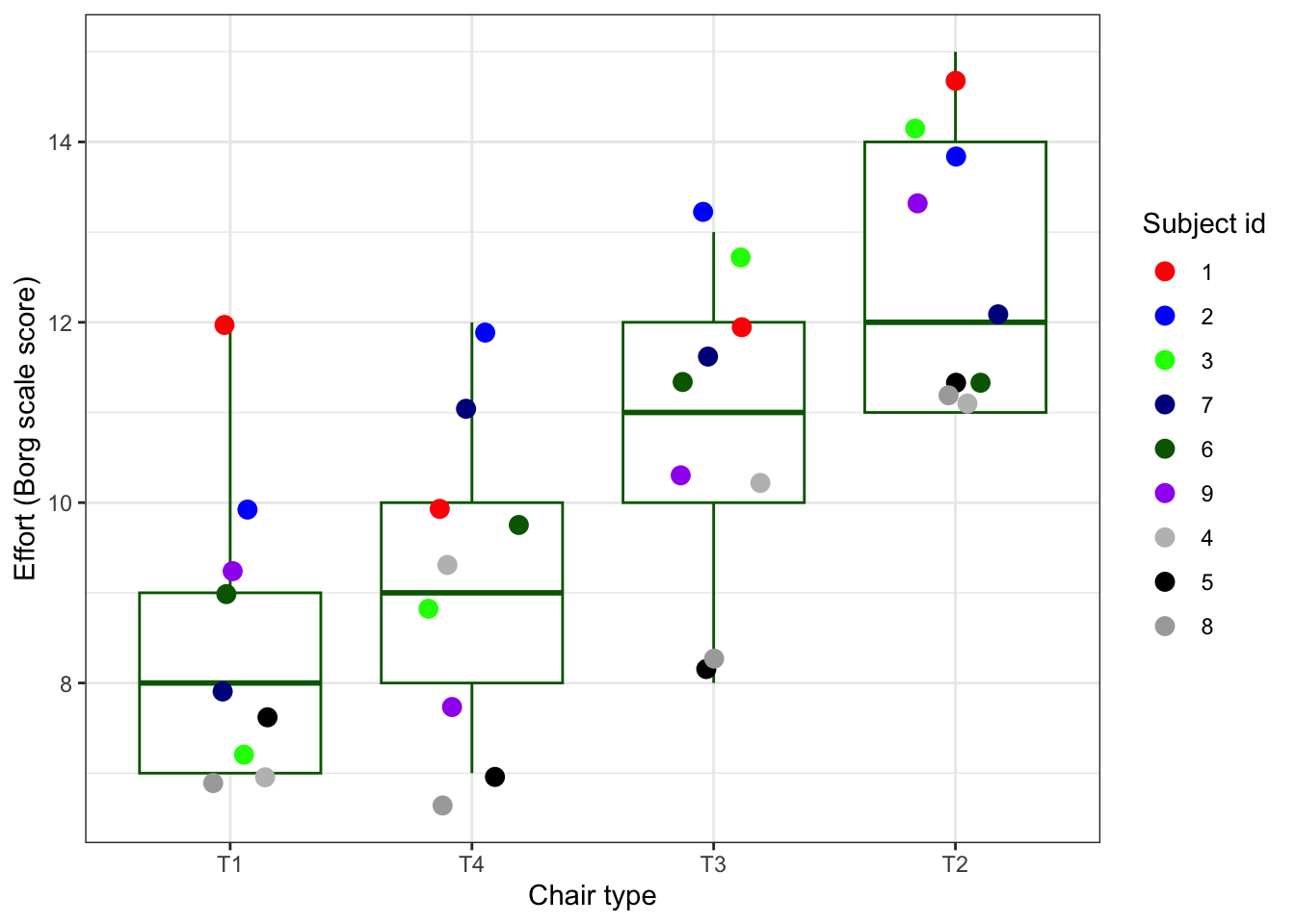
Exercise 4
Mind the variability per subject, what do you see?
- Can you say something about within-subject variability (note ‘Mister Blue’)?
- Can you say something about between-subject variability (note ‘Mister Green’, vs ‘Mister Black’)?
- Which chair type takes, on average the biggest effort to arise from?
- Looking at the code, why do you think the x-axis is not displaying the
Chair typein a numeric order?
4.5.5 The statistical questions
When we look at the scientific question and the data, we can deduce a number of statistical questions
- Which chair type takes, on average the biggest effort to arise from?
- What model would best capture the variability we see in the data, how would we reflect for example the inter-personal variability we observed in the exercise above, in a model
- Do individual (within subject) differences play a role in appointing a average score to a chair type? (MEM, random effects)
- Does variability between subjects play a role in determining the ‘best’ chair type (ANOVA / MEM, confidence intervals)
- What numbers can we appoint to the questions above? Numbers in statistics are usually called parameters.
4.5.6 The statistical model
Statistical models (in R) can be specified by a model formula. The left side of the formula is the dependent variable, the right side are the ‘predictors’. Here we include a fixed and a random term to the model (as is common for mixed-effects models). The fixed and random terms in the model are terms that reflect here the randomization (over persons) and the inter-person variability we observe in the data.
ergo_model <- lme(
  data = ergoStool, # the data to be used for the model
  fixed = effort ~ Type, # the dependent and fixed effects variables
  random = ~1 | Subject # random intercepts for Subject variable
)
We choose here to allow each volunteer to have its own curve, that has an intercept with the y axis. For sake of simplicity we assume the curves run parallel, so we assume a fixed slope. In more complicated designs we could also include a random slope, that allows the curves to vary in slope. This can be interpreted as that the effect of Chair type on Effort is not equal for each combination of Chair type and subject.
Lets see if the assumption of fixed slope holds:
plot_ergo_slopes <- ergoStool %>%
  ggplot(aes(x = reorder(Type, effort), y = effort)) +
  geom_jitter(aes(colour = reorder(Subject, -effort)),
              width = 0.2, size = 3) +
  geom_smooth(aes(group = Subject, colour = Subject), method = "lm", se = FALSE) +
  scale_colour_manual(
    values = c(
      "red","blue",
      "green", "darkblue",
      "darkgreen", "purple",
      "grey", "black", "darkgrey")
    ) +
  ylab("Effort (Borg scale score)") +
  xlab("Chair type") +
  guides(colour=guide_legend(title="Subject id")) +
  theme_bw()
plot_ergo_slopes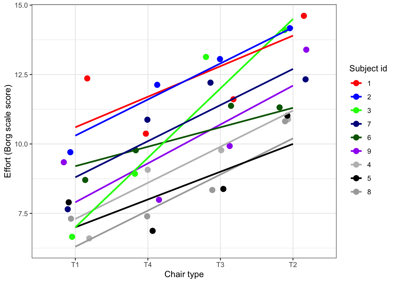
What do you think? Is the assumption for a fixed slope defensible?
4.5.7 The statistical results
| Value | Std.Error | DF | t-value | p-value | |
|---|---|---|---|---|---|
| (Intercept) | 8.5555556 | 0.5760123 | 24 | 14.853079 | 0.0000000 |
| TypeT2 | 3.8888889 | 0.5186838 | 24 | 7.497610 | 0.0000001 |
| TypeT3 | 2.2222222 | 0.5186838 | 24 | 4.284348 | 0.0002563 |
| TypeT4 | 0.6666667 | 0.5186838 | 24 | 1.285305 | 0.2109512 |
4.5.8 Model diagnostics
- Diagnostics of a fitted model is the most important step in a statistical analysis
- In most scientific papers these details are lacking
- If no model diagnostics are present, the question arises: Did the authors omit to perform this step? Or did they just not report it?
- If you do not want to include it in your paper, put it in an appendix, or even better, online together with the dat and the analysis script(s)!
A residual plot shows the ‘residual’ error (‘unexplained variance’) after fitting the model. Under the Normality assumption standardized residuals should:
- Be normally distributed around 0
- Display no obvious ‘patters’
- Should display overall equal ‘spread’ above and below 0 (‘assumption of equal variance’)
The details of the residual plot and the underlying theory do not matter much here. You only have to look at the plot and assess whether tha above assumptions are met or not.

4.5.10 The conclusions in a plot
We will spend a Masterclass on creating ‘publication grade’ graphs. Here is one that you could find in a paper about the ergoStool experiment and the analysis we did above.
# install.packages("ggsignif")
library(ggsignif)
p_values <- result$tTable %>% as.data.frame()
annotation_df <- data.frame(Type=c("T1", "T2"),
                            start=c("T1", "T1"),
                            end=c("T2", "T3"),
                            y=c(16, 14),
                            label=
                              paste("p-value:",
                              c(
                              formatC(
                                p_values$`p-value`[2], digits = 3),
                              formatC(
                                p_values$`p-value`[3], digits = 3)
                              )
                            )
                          )

set.seed(123)
ergoStool %>%
  ggplot(aes(x = reorder(Type, effort),
             y = effort)) +
  geom_boxplot(colour = "darkgreen",
               outlier.shape = NA) +
  geom_jitter(aes(
    colour = reorder(Subject, -effort)),
    width = 0.2,
    size = 3) +
  scale_colour_manual(
    values = c(
      "red", "blue","green",
      "darkblue", "darkgreen",
      "purple", "grey", "black",
      "darkgrey")) +
  ylab("Effort (Borg scale score)") +
  xlab("Chair type") +
  guides(colour=guide_legend(title="Subject id")) +
  ylim(c(6,20)) +
  geom_signif(
    data=annotation_df,
    aes(xmin=start,
    xmax=end,
    annotations=label,
    y_position=y),
    textsize = 5, vjust = -0.2,
    manual=TRUE) +
  theme_bw() -> plot_ergo
plot_ergo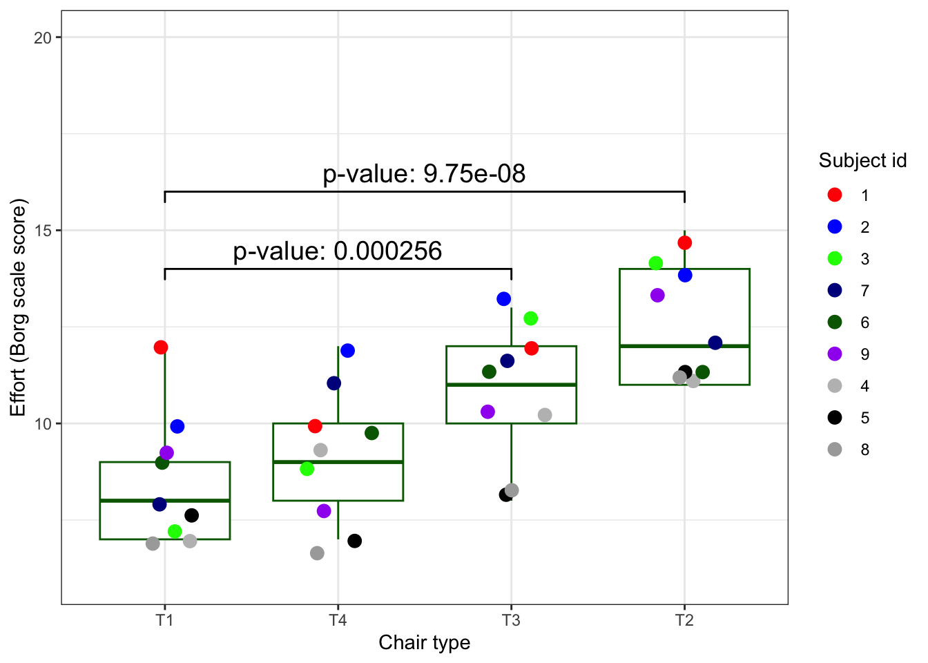
4.6 Example; The Open Science Framework OSF
To enable and facilitate the practice op Open Science, there are a number of organizations and foundations that support researchers. Below are a few examples. It is helpful to know about them if you are looking for places to get data, share data and code and to find good practices and examples.

\(Reproducible\ Science = P + D + C + OAcc + OSrc\)
OSF has it all
\(P = Publication\), \(D = Data\), \(C = Code\), \(OAcc = Open\ Access\), \(OSrc = Open\ Source\)
4.6.1 OSF - Reproducible Project: Psychology
- 100 publications in Psychology journals
- Results from half of these publications could be reproduced
- Full access to P, D and C in OSF
- The publication is not published in an OAcc journal but:
- The submitted manuscript is available in OSF
- The R code used is available in OSF
4.6.2 Another journal that supports Open Science is F1000 Research
The journal can be found here. Have a look at the special Bioconductor channel: https://f1000research.com/gateways/bioconductor
Portfolio assignment
Maak opdracht 4b van de portfolio-opdrachten.
4.7 Resources
https://www.displayr.com/what-is-reproducible-research/
https://book.fosteropenscience.eu/en/02OpenScienceBasics/04ReproducibleResearchAndDataAnalysis.html
CC BY-NC-SA 4.0 This work is licensed under a Creative Commons Attribution-NonCommercial-ShareAlike 4.0 International License. Unless it was borrowed (there will be a link), in which case, please use their license.