Extra Primer to R for data science
The GUI problem
Most people would agree that this seems to be a good practice. However, many people use GUI based software (graphical user interface). Citing Wikipedia, this is a “user interface that allows users to interact with electronic devices through graphical icons and audio indicator such as primary notation, instead of text-based user interfaces, typed command labels or text navigation.” So basically, any program that you use by clicking around in menu’s, or using voice control etc, for data science this could for instance be Excel.
However, how would you ‘describe’ the steps of an analysis or creation of a graph when you use GUI based software?
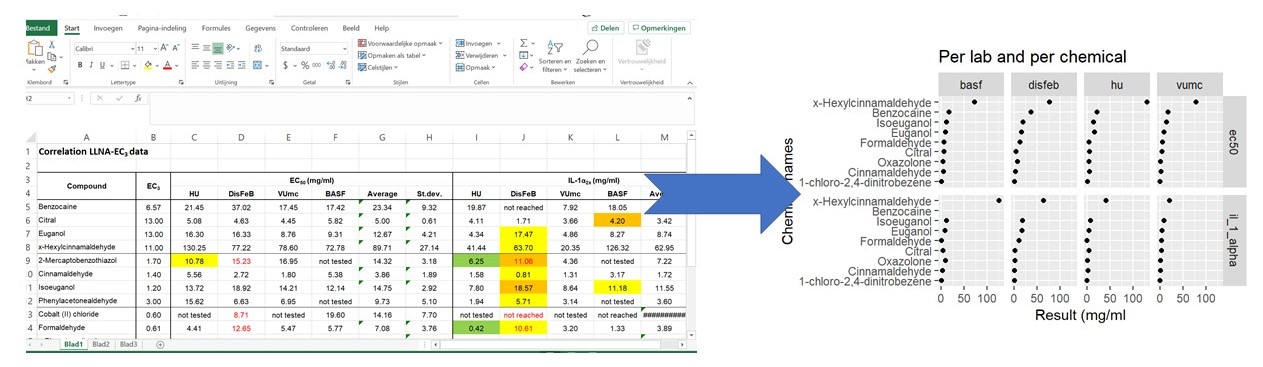
**The file “./Rmd/steps_to_graph_from_excel_file.html” shows you how to do this using the programming language R.
Maybe videotape tiktok-record your process and add .mp4 to your paper? Type out every step in a Word document? Both options seem rather silly. This is actually really hard!
This is why so many researchers are using code to analyse their data. If you do, just make sure you keep the code with the data. If you don’t, make sure you precisely keep track of every step you take, in a separate text document.
Using code
In Brown & Kaiser (2018), the authors write an important note on science that drives Reproducible Research:
“…in science, three things matter:
the data,
the methods used to collect the data […], and
the logic connecting the data and methods to conclusions,
everything else is a distraction.”
This means that in practice, when we adhere to the Reproducible Research principles, we can reproduce the analysis and the results from a data analysis in a paper when we:
- Are sure that the data is exactly the same as the data used by the authors of the paper
- We have the exact methods used to do the analysis
- We have a reproducible analysis environment (meaning we use the same software and/or settings)
This sounds trivial, but really is not. This also leads to the conclusion that using software that depends on a graphical user interface is not really compatible with Reproducible Research. We are going to illustrate this with a small exercise. This exercise is meant as a primer to get you to consider using a programming language to do data analysis. Although the authors are quite agnostic when it comes to programming for data science. Meaning they could basically learn every language because of prior knowledge. They both howver, prefer working with R. We will give something of a primer on R in part 3 of this short course. Although both authors are adept programmers a word of warning is appropriate here: Learning to program is hard. It need practice, discipline and patience. Frustration and errors are an integral part of learning how to and doing programming. In the long run, you will be able to ‘cash’ on your investments, but it is not an easy win and usually you will also be opposed by some (or many if you are unlucky) in your academic environment. Learning how to use a programming language to solve analytic problems, to generate visualizations and to write your future publications (yes you can!) does have the advantage that you will be able to integrate the Reproducible Research principles in full in your daily work as a scientist. More on this later.
Exercise; Recreating a graphs and recording the steps, given the data and the result
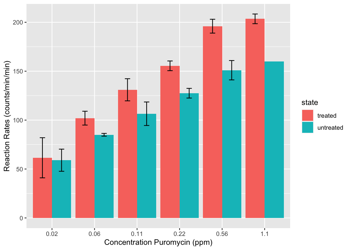
Spend 5-10 minutes recreating the graph below from the dataset steps_graph_excel.csv here. Record at least 10 steps that you would need to recreate your version of this graph.
Data Source
This dataset is part of the base-R installation in the {datasets} R-package as the Puromycin dataset-object.
## ── Attaching packages ─────────────────────────────────────── tidyverse 1.3.1 ──## ✔ ggplot2 3.3.6 ✔ purrr 0.3.4
## ✔ tibble 3.1.7 ✔ dplyr 1.0.9
## ✔ tidyr 1.2.0 ✔ stringr 1.4.0
## ✔ readr 2.1.2 ✔ forcats 0.5.1## ── Conflicts ────────────────────────────────────────── tidyverse_conflicts() ──
## ✖ dplyr::filter() masks stats::filter()
## ✖ dplyr::lag() masks stats::lag()## conc rate state
## 1 0.02 76 treated
## 2 0.02 47 treated
## 3 0.06 97 treated
## 4 0.06 107 treated
## 5 0.11 123 treated
## 6 0.11 139 treated
## 7 0.22 159 treated
## 8 0.22 152 treated
## 9 0.56 191 treated
## 10 0.56 201 treated
## 11 1.10 207 treated
## 12 1.10 200 treated
## 13 0.02 67 untreated
## 14 0.02 51 untreated
## 15 0.06 84 untreated
## 16 0.06 86 untreated
## 17 0.11 98 untreated
## 18 0.11 115 untreated
## 19 0.22 131 untreated
## 20 0.22 124 untreated
## 21 0.56 144 untreated
## 22 0.56 158 untreated
## 23 1.10 160 untreated