Lesson_01 - The research cycle

Learning objectives

The student is able:

To use Rstudio and bash commands to organize data files on a server
To explain the different types of research questions
To apply the research cycle to answer a research question
To apply the data analysis workflow for data analysis
To choose the right type of graphs for data visualization

Data management

An important part of data analysis is how to label and store and organize your data files. Similar to lab work, you label all your buffers, chemicals and tubes. After your experiment you put everything back to their appropriate save storage place. In data analysis we will do the same.

Storage: linux server
Organisation: what is your folder structure on the server + file names
Accessibility: who has access to your data (only you and the teachers)
Sharing: how to share your data with other researchers
Safety: raw data, data back-up, how to prevent losing data
Security: How to prevent that non-authorized persons have access to your data

Data analysis in Rstudio

During this course we will use a HU linux server in combination with Rstudio for data management and analysis. RStudio is a graphical user interface for the R programming language and can also contains a terminal to execute bash commands

To log in to the HU server, go to the following https:

https://bid.rstudio.hu.nl

Each student will have a (private) home directory (= folder) on the server (Figure 1)

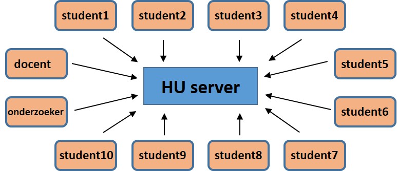
Figure 1: Each student has its own workspace on the server

When you log in and go to the terminal you always end up in your home directory (Figure 2). The files on the server are listed in the right lower panel under the “Files” tab. Here, you can create, copy, delete folders and data files (Figure 2).

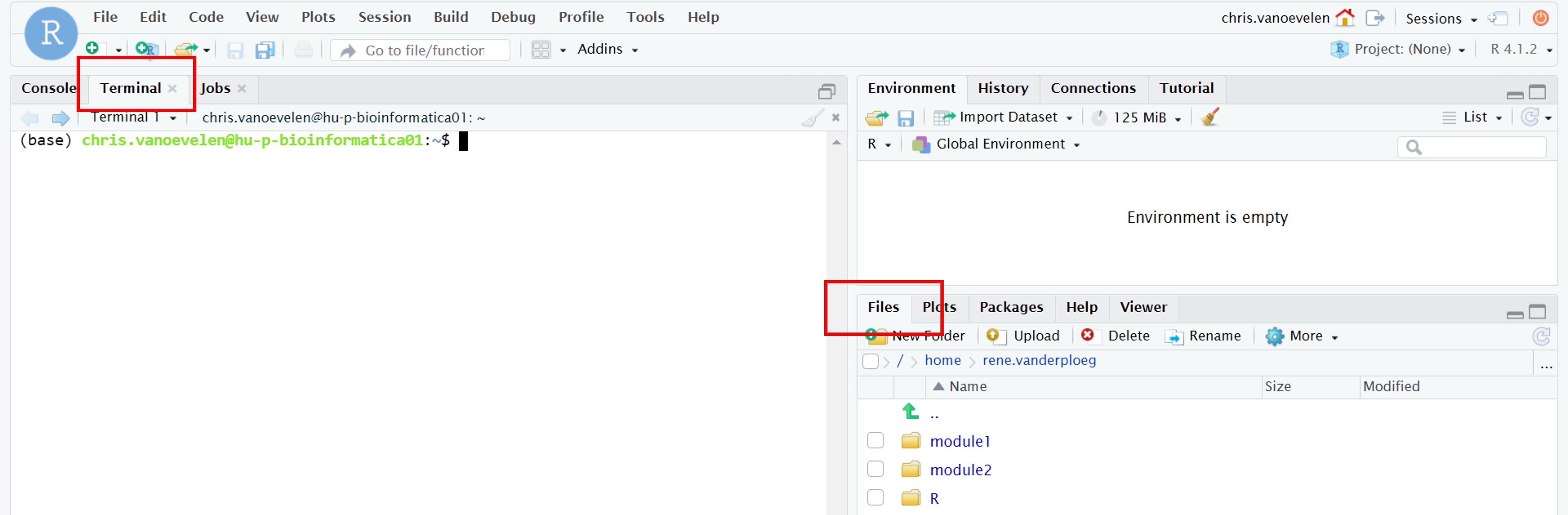
Figure 2: Rstudio interface with tabs for the terminal (left red box) and files (right)

Click on the terminal tab. You will now see the bash terminal.

The bash terminal is the interface between you and the server. In the terminal we can type bash commands (Figure 3) to see which files are present on the server, to make new folders, to move and copy files and to analyse data files and much much more.

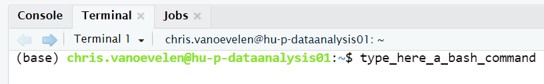
Figure 3: Rstudio terminal and bash commands

We can also write our own bash programs to automate tasks! There are many bash commands. Bash commands have options to modify the output of the command. To see which options are associated with a bash command type –help behind a bash command:

name_of_bash_command --help

During this course we will introduce some bash commands to organize, manipulate and analyse our data. Another great source for tutorials on bash commands can be found here

IMPORTANT: we recommend to perform all data management steps using bash commands in the terminal in stead of the Rstudio folder options in the right lower panel. We will extensively use the terminal during this course and with good practice you will learn how to use it. Instruction for data management will only be given with bash commands with the exception of data transfer (see below). Be aware that bash is case sensitive: “linux” means something different as “LINUX”!

Bash: make directory

When you log-in the server you start in your home directory which is empty except for a few (hidden) system files. The first step is to create a folder for each lesson of the course. To make a new directory on the server use the mkdir commmand (= make directory) followed by the name of the new directory:

mkdir lesson_1

We have 10 lessons so we have to repeat this command nine times. Doesn’t Sound like a good idea. What if you have to make a hundred directories!

There are several golden rules in programming, one of which is that we will never repeat the same command for the same task. The advantage of bash commands is that they come with extra options. Here we can use a special trick to generate all directories at once:

mkdir lesson_{1..10}

or if you have already made directory lesson_1:

mkdir lesson_{2..10}

Bash: list

To see which files and directories are present in your current directory you use the ls command (=list). The ls command shows all sub-directories and files in a directory:

ls

If we want extra information about the sub-directories, for example the size, we can use options (arguments) associated with the ls command:

ls -lh

The -l option shows the content of the folder as a list and the -h option stands for human readable to format the output of the list

For a list of all options associated with the ls command

ls --help

Bash: print work directory

Before we start navigating and go to the sub-directories containing our data, it is useful to learn the pwd command (print working directory). This command shows you in which folder you are currently working (Figure 4):

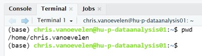
Figure 4: Bash pwd command

The example shows the home directory of chris.vanoevelen:

/home/chris.vanoevelen/

If you perform the pwd command you will see

/home/your_home_directory/

your_home_directory = either your name or your student number

Bash: change directory

The next step is to navigate to directories with the cd command (change directory). To change directory we have to “tell” the cd command where the directory is located on the server. The location of a file or directory is called a path or pathname

Generally, the cd command works as follows:

cd path_to_directory

Let’s say there is the following hierarchical (sub)directory structure in your home directory (Figure 5):

dir1.2 is within dir1.1, which is in dir1, which is in your home directory
dir2.2 is within dir2.1, which is in dir2, which is in your home directory

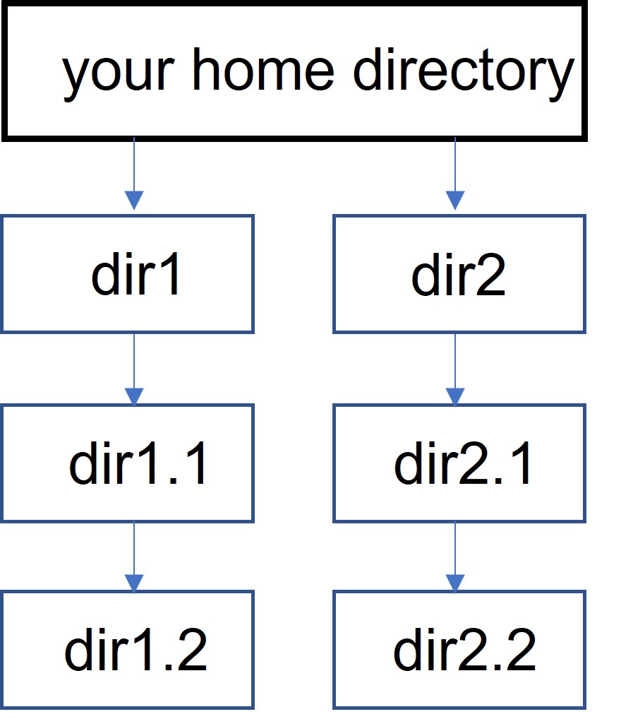
Figure 5: Hierarchical directory structure

There are two ways to point to files or directories on the server:

Absolute path: your pathname always start from the root directory (/home/your_home_directory/)
Relative path: your pathname always start from your working directory ( = directory where you are currently located)

Example 1:

Your working directory is dir1.1 and you want to go to dir1.2 (Figure 5)

Absolute path:

Your starting point is your home directory so you go three directory down in the hierarchy (see Figure 5)

cd /home/your_home_directory/dir1/dir1.1/dir1.2

There is also a symbol for your home directory which is the ~ sign. The ~ symbol means /home/your_home_directory. Thus, the above path can also be written as:

cd ~/dir1/dir1.1/dir1.2

Relative path:

Your working directory is dir1.1 so you go one directory down in the hierarchy (see Figure 5)

cd dir1.2

Example 2:

Your working directory is dir1.1 and you want to go to dir2.1 (Figure 5)

Absolute path:

Your starting point is your home directory so you go two directories down in the hierarchy (see Figure 5).

cd ~/dir2/dir2.1

Relative path:

Your working directory is dir1.1 so you go two directories up in the hierarchy to go to the home directory. From there you can select dir2 and its sub-directories (see Figure 5). To go one folder up in the hierarchy, the path is written as ../ . To go two folder up in the hierarchy we write ../../

cd ../../dir2/dir2.1

lesson_01_assignment

Use the cd command to go to directory lesson_1 within your home directory
What is now the path of your working directory

Shared directory

The data files for this course are located in a special shared directory which is accessible to all students.

To go to this directory:

cd /home/data/das3v22

From within this folder you can navigate to the other directories, for example the first lesson:

cd lesson_1

lesson_01_assignment

How many files are present in the shared folder /home/data/dasv22/lesson_1?
HINT: which bash command is used to show the contents of a folder?

If you want to go back to your home directory:

cd ~

Bash: copy

To copy data files and directories we use the cp command (copy)

Generally the cp command takes two arguments. The path of the files / folder that you want to copy (source) and the path of the destination directory.

cp path_to_file_or_folder path_to_destination_directory

For example, we want to copy file lesson_01_opdracht2_student.csv from the shared lesson_1 directory to the lesson_1 directory within your home directory

source: /home/data/das3v22/lesson_1/lesson_01_opdracht3_student.csv
destination: /home/your_home_directory/lesson_1

If our working directory is /home/data/das3v22/lesson_1 we can directly write the file name using a relative path

cp lesson_01_opdracht2_student.csv /home/your_home_directory_name/lesson_1

If we want to copy all files at once we can use the asterisk symbol * meaning all files present in a folder. This is a wildcard character. We will learn more about wildcard characters

cp * /home/your_home_directory_name/lesson_1

Rstudio File transfer

To upload data files from your computer to the server use the “Upload” button in the file panel:

Browse where you want to save the file on the server
Choose file to connect to your computer and select the file to be uploaded

To download files from the server to your computer use the More -> Export button in the file panel

IMPORTANT: All data files are located in the shared folder on the server. For each assignment copy the file from the shared folder to your home directory in the right sub-directory (lesson_1, lesson_2 and so on. From here you can download the files to your own computer.

Research questions

We are curious and want to know how things works. Research is all about asking interesting questions. In order to formulate a research questions we have to gather information of what is already known. Based on this information you start to phrase your research question, design an experiment and start measuring variables. A variable is anything that can be measured and vary between entities (research subjects) or in time. For example, variables are the number of DNA mutations in a genome, metabolite concentration in a urine sample, enzyme activity, blood pressure, weight, length and so on.

There are different types of research questions:

Exploratory / descriptive:

Descriptive research questions provide answers on existing features of the research subjects (we don’t know what causes these features, we only describe them)

What is the average blood pressure of diabetics patients?
How many genes are present in the human genome?
How long is the cell cycle of a certain eukaryotic cell line?
Which P53 mutation are present in a leukemic cell line?

Correlation: is there a correlation between two variables?

Correlation research questions provide answers on the relationship between two variables in a natural environment. The researcher does not manipulate the variables. Importantly, we can’t state that an increase of variable 1 causes an effect (increase or decrease) of variable 2. Because the effect can always be caused by another unknown variable.

Is there a correlation between weight and blood pressure in diabetics patients?
Is there a correlation between the size of the genome and the number of genes?
Is there a correlation between type of growth media and the length of the cell cycle?
Is there a correlation between the type of P53 mutation and the prognosis of breast cancer?

Comparative: is there a difference in the level of what is being measured between a reference group and group(s) that are experimentally manipulated

Comparative research questions provide answers on cause and effect. As a start groups are created that are as similar as possible (for example rats or mouse of equal weight, sex and age). One group is not treated and the other group(s) are experimentally manipulated (for example expoure to a chemical). Therefore it is assumed that the observed effects in the experimental group are only caused by the experimental manipulation.

Is there a difference in blood pressure between diabetics mice and control mice?
Is there a difference in the number of gene transcripts between protein coding and non-coding genes?
Is there a difference in the length of the cell cycle between cells grown with low or high levels of glucose?
Is there a difference in the type of P53 mutations between cells originating from a breast tumor or leukemic cells?

The research cycle

To obtain an answer to our research questions we follow the steps of the research cycle (Figure 6). As mentioned above we first gather existing information on the subject and formulate our research questions and sub-questions. The next step is to transform your research questions into an hypothesis and related predictions which can be tested by either descriptive, correlational or experimental research.

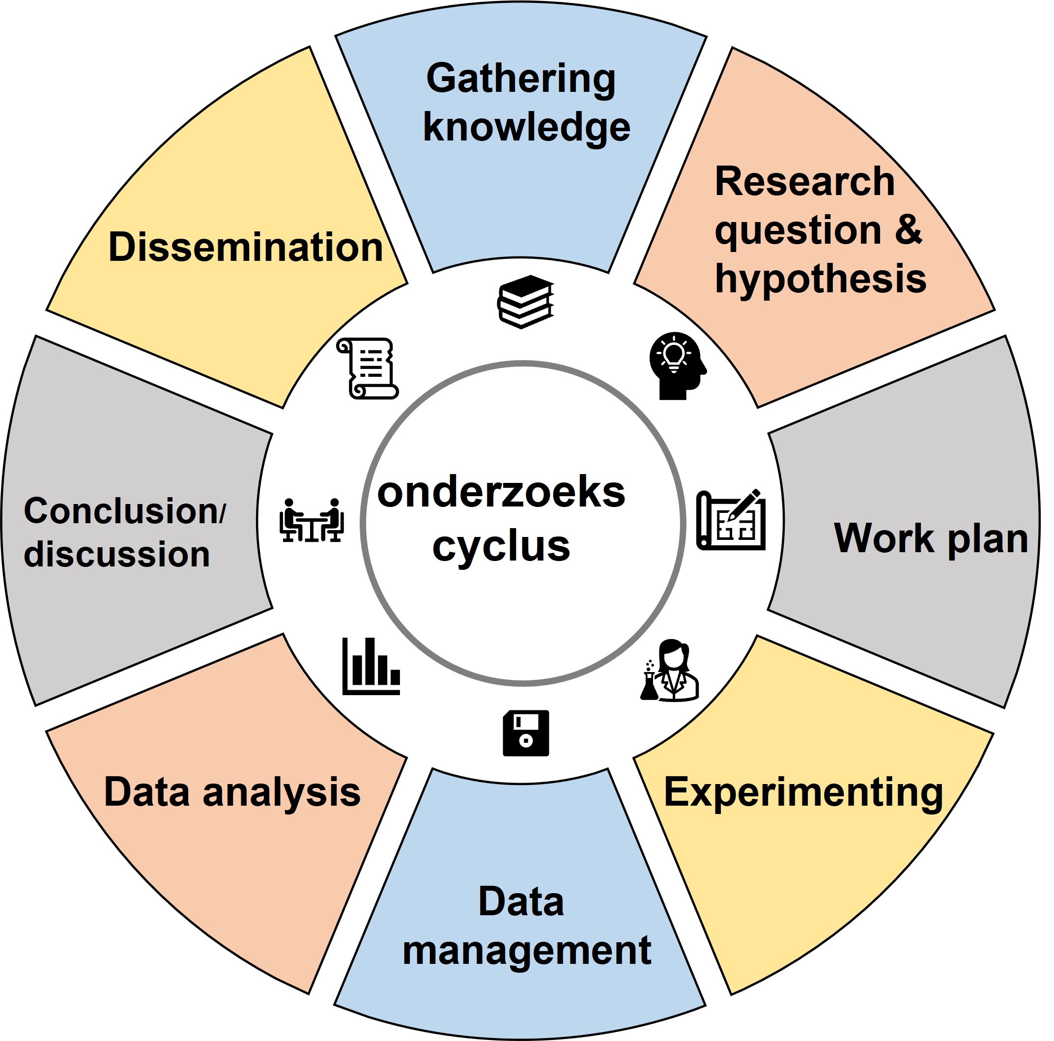
Figure 6: Research cycle

In the next 10 lessons you we’ll learn how to answer research questions using the research cycle with a focus on gathering information and data analysis . The research questions cover all types of biological experiments with different levels of biological data:

DNA -> RNA -> protein -> cell -> tissue -> physiological -> organism

IMPORTANT: In the next sections the different steps of the research cycle will briefly be explained. Without an in depth understanding of the research cycle you can’t successfully finish this course. It is therefore very important to thoroughly read and understand the next sections.

Experimental design

A critical part of the research cycle is to properly design your experiment. This will ultimately determine the statistical analysis that can be performed and how reliable your conclusions are. If your experiment is not well designed you can’t conclude anything at all (and unfortunately, this is often the case!). In the next section we will discuss some aspects of experimental design which are important to successfully analyse your data

Experimental and outcome variables

Generally a comparative scientific experiment will consist of three parts (Figure 7).

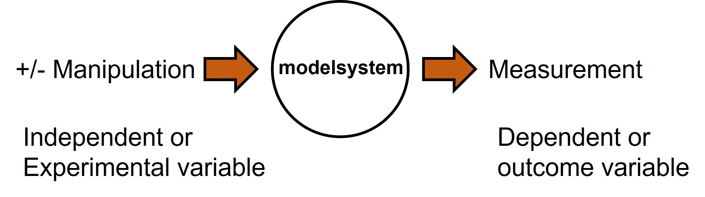
Figure 7: experimental and outcome variables in experimental design

In a comparative experimental design the researcher decides which variable to change in the model system (i.e. model systems can be humans, plants, fruitflies, cancer cells, genome and so on) and tries to keep all other variables equal between the groups. The variable that is changed between groups is called the independent or experimental variable (yet another name is predictor variable). The variable that will be measured is called the dependent or outcome variable.

NOTE: When addressing a descriptive research question we still have to determine our model system and the outcome variable i.e. what will be measured? When addressing a correlational research question we also have to think about the modelsystem and which two variables will be measured

One-way or two-way experimental design

An experimental design with one experimental variable is called a one-way setup. For example, a researcher wants to test growth rates (outcome variable) of cancer cells (model system) after exposure to a potential drug (experimental variable). Even if the researcher uses different concentrations we call it a one-way setup because there is still one experimental variable but with different values.

A two-way experimental set up includes two experimental variables. For example the researcher could try the drug on different cellines:

1st variable: drug (using one or different concentrations)
2nd variable: cell type

A typical two-way experimental set up is shown in Figure 8

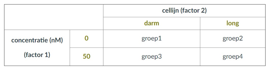
Figure 8: crosstable of a two-way design

Population vs sample:

Ideally you want to measure a variable of the population. For example, the average hematocrit value of all healthy women in the Dutch population is 0,41 L/L. A numerical description of a variable from a population (in this example 0,41 L/L) is called a parameter. By measuring the population your results and conclusions are generally applicable and can give support for existing theory or new ones. However, it is not always possible to measure the population! It could be too expensive, takes too long or test animals must be sacrificed to measure your variable. It could also be unethical, for example to study brain patterns of all children watching horror movies.

If it’s not possible to study the population (and most often this is the case) we will make use of a sample. A sample should always be representative of the population (but how do we know this?). For example, a sample of the hematocrit level in healthy Dutch women can give a value of 0.45 L/L (this deviates from the actual population parameter of 0.41 L/L, see text above). A numerical description of a variable from a sample (in this case 0,45 L/L) is called a statistic. By using inferential (or inductive) statistics the population parameter can be estimated using a sample statistic. In other words, with the help of a sample, which is only a small part of the population we try to say something about the whole population. The central question is … how accurate is my sample and therefore my prediction?

Sample size

How many elements should minimally be in your samples to observe an effect that actually exists in the population. A sample is always a representation of the population and the bigger the sample size the better the representation. If your sample size is too low, your study is under-powered. This will increase the chance that you can’t show a true effect with your samples that exists in the population. This is very important because you invest a lot of time, expensive chemicals and possibly test animals as your model system (think about the ethical aspects of your experimental design) to answer your research question. But because of the small sample size on beforehand you were never able to do so! But a big sample is more costly, takes more time and when test animals are involved also unethical. So what is the right size of the sample to show a real effect that exist in the population? Or to be sure that an effect doesn’t exist in a population.

Biological and technical replicates

Biological replicates: measurements of biologically distinct samples that show biological variation
Technical replicates: repeated measurements of the same sample (to measure background signal associated with the equipment and the protocols)

Paired or unpaired experimental set-up?

The holy grail of a comparative experimental setup is to keep all variables equal except for the experimental factor. Preferentially, a paired experimental set-up is used in which the same subjects are measured twice: before and after the experimental manipulation (Figure 9). This way each subject serves as its own control and reduces variation between the (paired) measurements.

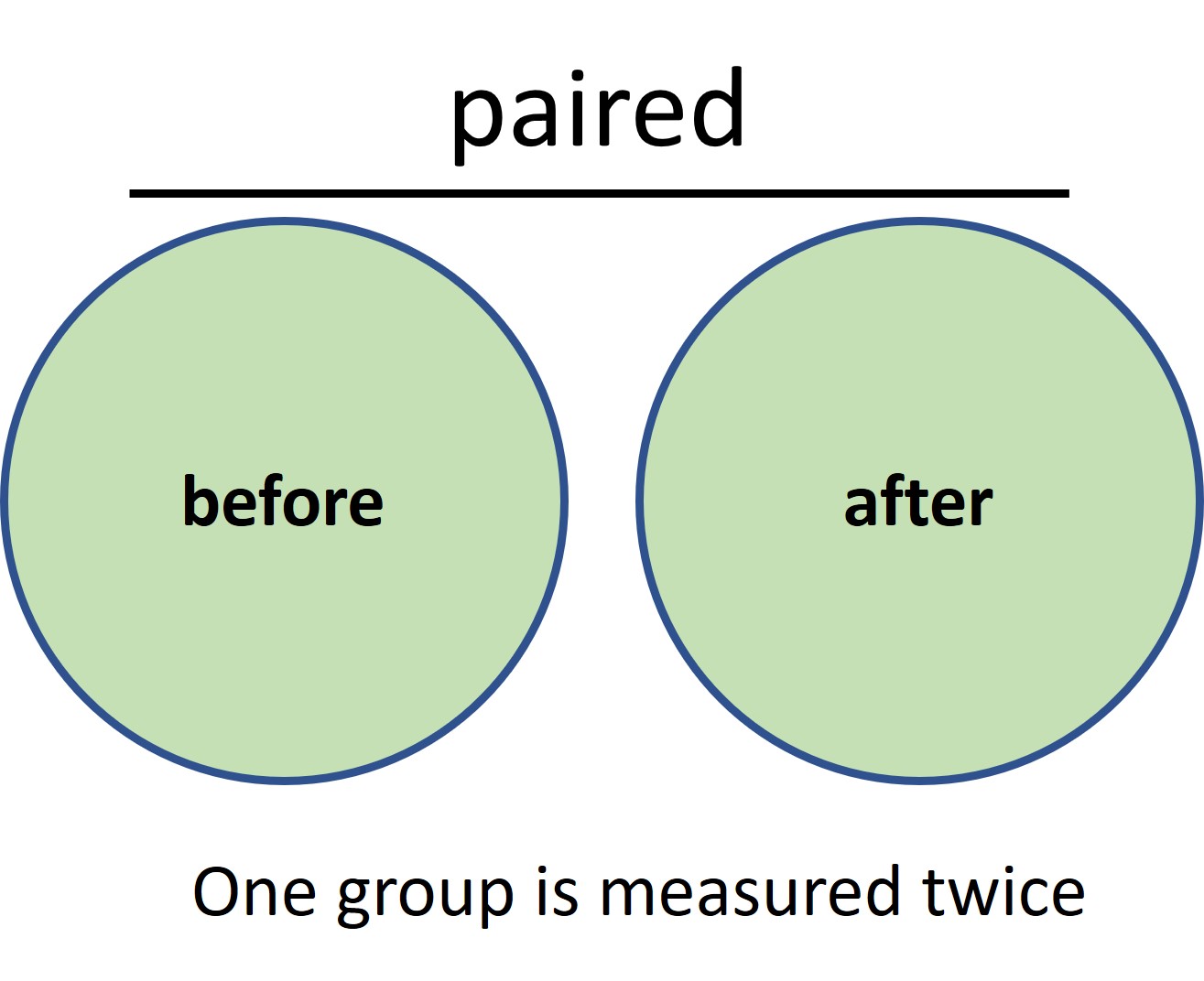
Figure 9: paired experimental set-up

However, it is not always possible to measure twice on the same subject. What if the subject has to be sacrified to collect DNA, tissues or cells. Then the ‘after’ measurement is not possible and an unpaired experimental set-up is required (Figure 10).

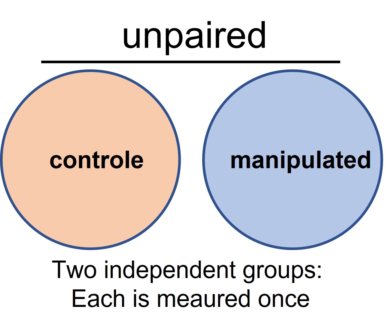
Figure 10: unpaired experimental set up

At least two (or more) groups are created. In an unpaired experimental setup one group serves as the reference group (or control group) and the other groups is experimentally manipulated. Before the start of the experiment it is assumed that groups are more or less equal, for example the same genetic background. However we are always dealing with natural variation! Thus before any experimental manipulation we expect to measure differences between the groups because of natural variation. We want this background signal as low as possible (because we haven’t started the experiment yet). After the experiment we measure the difference between the groups and calculate if this difference is higher then the background signal. Because natural variation is smaller in paired experiments as compared to unpaired experiments it is easier to show whether the manipulation has an effect on the outcome variable in paired experiments.

Number of variables to measure

In principle you can measure as many variables as possible. For example medical records of patients not only contain information about age, gender, length and weight but also for example, acquired diseases, mental state, blood pressure, number of visits to the general practitioner, medicine use, smoking and so on. These kind of records are used for correlation analysis to study the relationship of life style choices on mental en physical health.
Another example is transcriptome analysis. Using this techniques we can measure transcription levels of all genes of our cells of interest. Each gene is considered a variable meaning that if we would compare two conditions we can perform twenty thousands Student’s t-test!

Performing multiple statistical tests increases the chance of finding false positives which are meaningless. This is called data dredging. There are many spurious correlations which just happen by chance.

Level of measurement

How you’re going to measure your variable determines the level of measurement. In most cases a measuring device will output some numbers. But what if you want to count the number of dead or alive round worms after exposure to some chemical. Or what about imaging data to monitor the morphology of brain tissue after a seizure. How to deal with this kind a data?

It is important to know on beforehand what type of data will be generated. There are 4 levels of measurements based on whether the data is qualitative or quantitative. The level of measurement determines the statistical test that can be performed on the data. The least informative data is nominal whereas ratio data is the most informative. .

Qualitative data:

nominal: categorical data which can not be ordered; gender, blood type, dead or alive
ordinal: categorical data which can be ordered; quality scores (bad, neutral, good)

Quantitative data:

interval: numerical data with no absolute null point ; temperature in Celcius
ratio: numerical data with an absolute null point; concentration, weight, age

IMPORTANT: The type of research question, experimental setup and scale of measurement determines the type of statistical analysis you can perform.

Data analysis workflow

After we’ve obtained the experimental data we’ll have to perform data analysis

Data analysis can be divided into several steps.

Data import: load data into data analysis software (Excel, JASP, bash, R)
Data inspection: how is the data organized and what is being measured
Data organisation and transformation: cleaning up the data, restructuring the data, modifying rows and columns, perform additional calculations and so on
Descriptive statistics: summarize and graph the characteristics of a sample (mean, median, stdev)
Inductive statistics: draw conclusions from samples and generalize these conclusion to the population from which the samples were drawn
Communication: visualization of data using graphs / data reports

IMPORTANT: These steps will provide a general framework for all your data analysis during this course and future work.

Conclusion, discussion

After the data analysis we draw conclusions and discuss the data in the context of what is already known. Can we reinforce an existing theory or do we formulate an alternative explanation! New research questions will pop up and the research cycle starts all over again. This process is called the empirical research cycle. Theories are thus based on empirical evidence. A fundamental consequence of the empirical research cycle is that a theory must be falsifiable. It should always be possible to refute an existing theory. There is no absolute truth!! Research findings should always be interpreted in the simplest way (thus no far fetched explanations) and research findings are objective, free of any personal beliefs.

Communication and dissemination

After all you hard work and possible Nobel price winning research you want to communicate your results to the rest of the world. You either write a report, scientific paper, weblog or give a presentation (or any other type of communication). This way your results are available to the scientific community, so other researchers can interpret and discuss your results and start formulating new research questions

ALERT: Nowadays in media outlets we are experiencing an increase of strong claims based on anecdotal evidence (in contrast to empirical evidence) from self-proclaimed experts. Why this is useless is explained here. As a critical researcher never let you be tricked by anecdotal evidence!!

Graph types

An important tool to describe, explore and communicate your data are graphs. There are many different types of graphs and the type of graph you use depends on the experimental design and data types.

Bar chart: A graph that presents categorical (nominal) data with rectangular bars with heights or lengths proportional to the values that they represent. The bars can be plotted vertically or horizontally.
Scatter plot: A graph in which the values of two continous variables are plotted along x- and y-axes. The pattern of the resulting points could reveal any correlation present.
Box plot: A graph that shows the spread of quantitative data based on quartiles and outliers
Line chart:
A graph that connects data points with a line to show a (local) trend. The x-axis variable is continuous , preferably with similar intervals and most often involves time series but also concentrations, doses or any other increasing unit. For example, measurement of tumor size per week after treatment, or number of species per increasing area unit. Note: the x-values of a line graph should always be numeric !!
Histogram:
Representation of the distribution of numerical (continous) data. A histogram divides the x-axis into equally spaced bins and then uses the height of a bar to display the number of observations that fall in each bin.

Cancer incidence in the Netherlands

Before we start with (any) data analysis it is very important to decide which software to use. Most researcher still use Excel. Excel can be used for data organizing tasks and for exploratory figures. In this exercise we will use Excel to repeat and strengthen your Excel skills.

We will start with practicing the first 4 steps of the data analysis framework by answering questions about the incidence of different types of cancer in the Netherlands from 1989-2019. The data is obtained from De Nederlandse kankerregistratie (NKR). A description of the data can be found here.

lesson_01_assignment

Which cancer showed the highest incidence in the Netherlands in period 1989-2019?

Follow the steps below to answer the question

Import data file lesson_01_opdracht3_student.tsv in Excel (the data file extension = tsv. This stands for tab separated values)
Inspect the data (what are the experimental and outcome variables)
Organize the data in such a way that you can make a single (appropriate) graph
- What type of graph?
- What are the x-axis and y-axis variables?
- Label the x/y-axis
- Add an informative graph title

What is the answer on the research question?

Which two cancers showed the most % increase in incidence in 2019 relative to 1989?

Follow the steps below to answer the question.

Organize and transform the data to calculate the percentage increase from 1989 to 2019 for each type of cancer.
Organize the data in such a way that you can make a single (appropriate) graph
- What type of graph?
- What are the x-axis and y-axis variables?
- Label the x/y-axis
- Add an informative graph title

What is the answer on the research question?

Can you provide an explanation for the increase of the incidence for the two highest cancer types?

lesson_01_assignment

Which cancer showed the highest incidence in the Netherlands in male / female of age 20-24 in 2019

Import data file lesson_01_opdracht4_student.txt in Excel (the data file extension = txt. This means that the columns could be separated by anything. Most likely this is a tab separated data file)
Inspect the data (what are the experimental and outcome variables)
Organize and select the data in such a way that you can a make single (appropriate) graph - What type of graph?
- What are the x-axis and y-axis variables?
- Label the x/y-axis
- Add an informative graph title

What is the answer on the research question?

An example of anecdotal evidence is the statement that grandma smoked > 20 cigarettes a day for her whole life (let’s assume she started at the age of 30) and she became 90 years of age! Thus smoking isn’t that bad for your health!

Let’s translate this statement to a comparative research question: Does the chance of becoming 90 years old differ between woman who smoked heavily (> 20 cigarettes a day starting from 30 years of age) and non-smoking women?

With null hypothesis: The chance of becoming 90 years old is equal between woman who smoked heavily (> 20 cigarettes a day starting from 30 years of age) and non-smoking women.

If we want to answer our research question experimentally with an scientific experiment we’ll have to create 2 groups of women of about age 30. Let’s assume that the women in the groups are more or less equal in terms of length, weight and medical history. Thus, we assume no difference on beforehand between the two groups. One group serves as a control group and the other group is forced to smoke a minimum of 20 cigarettes a day. To control any other environmental factors we’ll lock them up and provide the same diet for all participants. As a measurement we count how many will reach the age of 90. Any difference we’ll measure between the two groups is attributed to the experimental factor (i.e. smoking) because as a start the two groups were more or less equal. I don’t think we’ll get away with this experimental set up!!

In order to address the aforementioned anecdotal statement we’ll have to make use of an alternative method. In this case we’ll use the observational research method. Using this method participants are being studied in their natural habitat. Thus, we can’t control all other environmental factors that possibly will affect the outcome of the experiment. In this case we can only make a correlation between smoking (how cigarettes a day) and the age of death.

Let’s translate our question to a correlational research question, for instance:
Is there a correlation between the number of cigarettes smoked per day and the age of death in women?

With null hypothesis: There is no correlation between (heavy) smoking and the chance of becoming 90 years of age in women

You could also define a descriptive research question, such as: how big is the chance for a heavy smoker to die before the age of 90?

Let’s investigate a few similar research questions.

The dutch “centraal bureau voor de statistiek” (CBS) monitors health in society. They have performed observational research in which they addressed the question whether life expectancy correlates with the level of smoking. Open the following link and read the article. The corresponding research communication lesson_01_opdracht5_roken_sterfte.pdf is present in the shared folder on the server.

lesson_01_assignment

Research question: how big is the chance for a heavy smoker to die before the age of 90? And non-smokers?

Download data from the link. Use the “DOWNLOAD CSV” button of the first figure
Import the data file in Excel
Inspect the data, to see how the data is organized
Recreate the graph with correct labels and an informative title (the same figure is present as Figuur 1 in the research communication)
Save the data as an Excel file named lesson_01_opdracht5.xlsx

What is the answer on the research question?

lesson_01_assignment

Is there a correlation between how many cigarettes a person (on average) smoked and age of death?

Import the data file lesson_01_opdracht6_student.txt in Excel
Inspect the data, to see how the data is organized
Organize and select the data in such a way that you can a make single (appropriate) graph
- What type of graph?
- What are the x-axis and y-axis variables?
- Label the x/y-axis
- Add an informative graph title

What is the answer on the research question?
What is the value of \(R\)? (note: not \(R^2\)) How would you interpret this value?