Lesson_09 - Statistics Part1

Learning objectives

The student is able:

To understand the concepts of population, statistic, sample, variable and parameter
To determine the distribution of a dataset
To perform descriptive statistics in JASP
To spot and remove outliers from a dataset
To assess whether the data is normally distributed
To execute parametric tests

Introduction

In the previous lessons we have mostly focused on how to retrieve biological information from public databases. In the next lessons we will extend our knowledge of statistics. Key concepts in statistics are:

Population: complete set of entities of which we want to measure a characteristic. A population can be finite (all 200 Dutch patients with a certain syndrome) or infinitely large (‘all healthy adult men’). The researcher defines the population and this depends on the research question. The population size is represented by N.

Sample: Random selection of entities from a population. A sample must be representative of the population and is used to make predictions about the entire population. The sample size is represented by n.

Parameter: Numerical representation that summarizes a property of a population such as the mean, dispersion, or fraction

A Statistic: Numerical representation that summarizes a property of a sample. A statistic is used to make a statement / estimate of the population parameter.

Variable: Anything that is measurable and gives different values between entities in a population (or sample) or within the same entity over time

lesson_09_assignment

Indicate which statistical concept is highlighted in purple. Choose from population, sample, parameter, statistic or variable.

A researcher wants to estimate the average height of women aged 20 or older. From a simple sample of 45 women, the researcher obtains an average sample height of 63.9 inches.
A nutritionist wants to estimate the average amount of sodium ingested by children under the age of 10. From a random sample of 75 children under the age of 10, the nutritionist calculates a sample mean of 2,993 milligrams of sodium consumed.

3.Nexium is a drug that can be used to reduce acid produced by the body and heal damage to the esophagus. A researcher wants to estimate the number of patients who take Nexium and recover from damage to the esophagus within 8 weeks. A random sample of 224 patients suffering from acid reflux disease taking Nexium is obtained and of those patients 213 were cured after 8 weeks.

A researcher wants to measure the number of lymphocytes per \(\mu\)l blood in persons with infectious mononucleosis (ziekte van Pfeiffer). Using a sample of 40 infected persons the researcher calculates an average value of 6000 lymphocytes per \(\mu\)l blood
A researcher wants to estimate the average number of lymphocytes per \(\mu\)l blood in persons with infectious mononucleosis (ziekte van Pfeiffer). Using a sample of 40 infected persons the researcher calculates an average value of 6000 lymphocytes per \(\mu\)l blood
A researcher wants to estimate the average number of lymphocytes per \(\mu\)l blood in persons with infectious mononucleosis (ziekte van Pfeiffer). Using a sample of 40 infected persons the researcher calculates an average value of 6000 lymphocytes per \(\mu\)l blood
A researcher wants to estimate the average number of lymphocytes per \(\mu\)l blood in persons with infectious mononucleosis (ziekte van Pfeiffer). Using a sample of 40 infected persons the researcher calculates an average value of 6000 lymphocytes per \(\mu\)l blood

Data analysis workflow

When we want to answer a research question, most often we take a sample from the population and start measuring characteristics (variables) of the entities within the sample. To reiterate your knowledge about experimental design go to lesson_01 -> Experimental design. After the experiment we have data. To draw a conclusion about your experiment it is essential to properly analyse your data:

The general framework for all your data analysis is:

Data import: load data into data analysis software (Excel, bash, R)
Data inspection: how is the data organized and what is being measured
Data organisation and transformation: cleaning up the data, restructuring the data, modifying rows and columns, perform additional calculations and so on
Descriptive statistics: summarize and graph the characteristics of a sample (mean, median, stdev)
Inductive statistics: draw conclusions from samples and generalize these conclusion to the population from which the samples were drawn
Communication: visualization of data using graphs / data reports

Descriptive statistics

Descriptive statistics displays or summarizes data in a meaningful way to reveal trends or patterns. Descriptive statistics of a sample always relate to the sample itself and do not describe the population of which the sample was derived from. Descriptive statistics allows us to present the data in a more meaningful way, allowing for easier interpretation of the data. Important characteristics of a data set are:

Central tendency
Dispersion
Type of correlation

Central tendency

Mode

Value that occurs most in a data set:

data set: 2 2 4 5 5 5 8 9 9 12

Mode = 5

Median

Middle value of a sorted data set. The median splits the data into two equal groups. Half of the of the values are below / above the median value:

data set: 2 2 4 5 5 5 8 9 9 9 12

Median = 5

Mean

Sum of all values divided by the number of values.

The symbol for the population mean: \(\mu\)
The symbol for the sample mean: x̄

The mean is the balance point of the data. The values below the mean have a similar total deviation from the mean as the values above the mean.

data set: 2 2 4 5 5 5 8 9 9 9 12

mean: 6,36

IMPORTANT: samples are summarized by a single value such as the mean value. This is called a single point estimate. How well represents this single value the complete data set? To assess how the mean fits the data we have to assess the dispersion of the data. How close / far are the single data points from each other and relative to the mean. If data values are close to each other the dispersion will be small. If the data points are scattered over a wide range of values the dispersion will be large:

data set 1: 27 28 29 30 32 34
data set 2: 17 18 19 30 42 54

Data set 1 and 2 have the same mean. But the dispersion of data set 2 is much larger.

Dispersion

To assess and quantify the dispersion of a data set the following statistics can be used:

Range:

Difference between the highest and the lowest value

data set: 2 2 4 5 5 5 8 9 9 9 12

range = 12 -2 = 10

Quantiles

Values of the data set that splits the sorted data set into a number of groups.

For example, quartiles split sorted data into four equal groups:

data set: 2 2 4 5 5 5 8 9 9 9 12

first quantile (25%) = 4
second quantile (50%) = 5
third quantile (75%) = 9

Inter-quartile range (IQR): difference between the third and first quartile:
In the example above the IQR: 9-4 = 5

A boxplot is used to show the distribution of the data using the quartiles (Figure 82) The 1st and 3rd quartiles form the bottom and top of the box, and the median is represented with a horizontal line in the box. The vertical lines below and above the box indicate highest and lowest values which are not outliers. A value is considered an outlier if the value exceed more than 1.5x the Inter-Quartile Range (IQR)

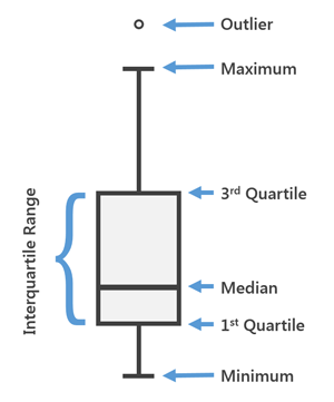
Figure 72: Interpretation of a Boxplot

Using a boxplot (or dot plot) we can also assess the distribution of the data (Figure 83). The distribution of your (continuous) data determines which statistical test can be performed (more about that later)

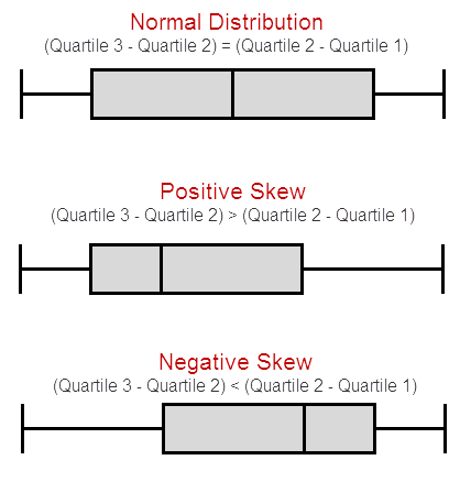
Figure 73: Boxplots and distributions

If a distribution is positively skewed, the mean is pulled upwards
If a distribution is negatively skewed, the mean is pulled downwards

Besides positive and negative skewed data we can also observe a bi-modal distribution (Figure 84). This happens when there is a sub-population within your population that has been sampled

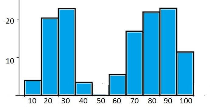
Figure 74: Bimodal distribution

For example, you sample diabetics patients but your variable ( = what has been measured) depends on normal and high blood pressure. Within your initial population there were two sub-populations

lesson_09_assignment

Copy data file lesson_09_opdracht2a.txt and lesson_09_opdracht2b.txt from the shared directory to your home directory -> lesson_09
Import the data files in JASP
Make a boxplot (Customizable plots)
Make a dot plot (Basic plots)

Interpret the histograms and dot plots of file lesson_09_opdracht2a.txt

Which group has the highest dispersion?
Are the groups normally distributed? Explain!

Interpret the histograms of file lesson_09_opdracht2b.txt

What is the type of distribution of group3 and group4? Explain! (see also figure 83)

Variance

The mean is a single point estimate representing all values (figure 85, mean = red line). How well the mean represents the data can be calculated with the variance.

Variance: average deviation of the data values relative to the mean.

To calculate the variance (Figure 85):

For each data value, calculate the difference with the mean (Figure 85, green arrows)
Square this difference
All squared difference are added up (= total squared deviation)
The total squared deviation is divided by
- size of population for the population variance
- sample size minus 1 (n-1) for the sample variance

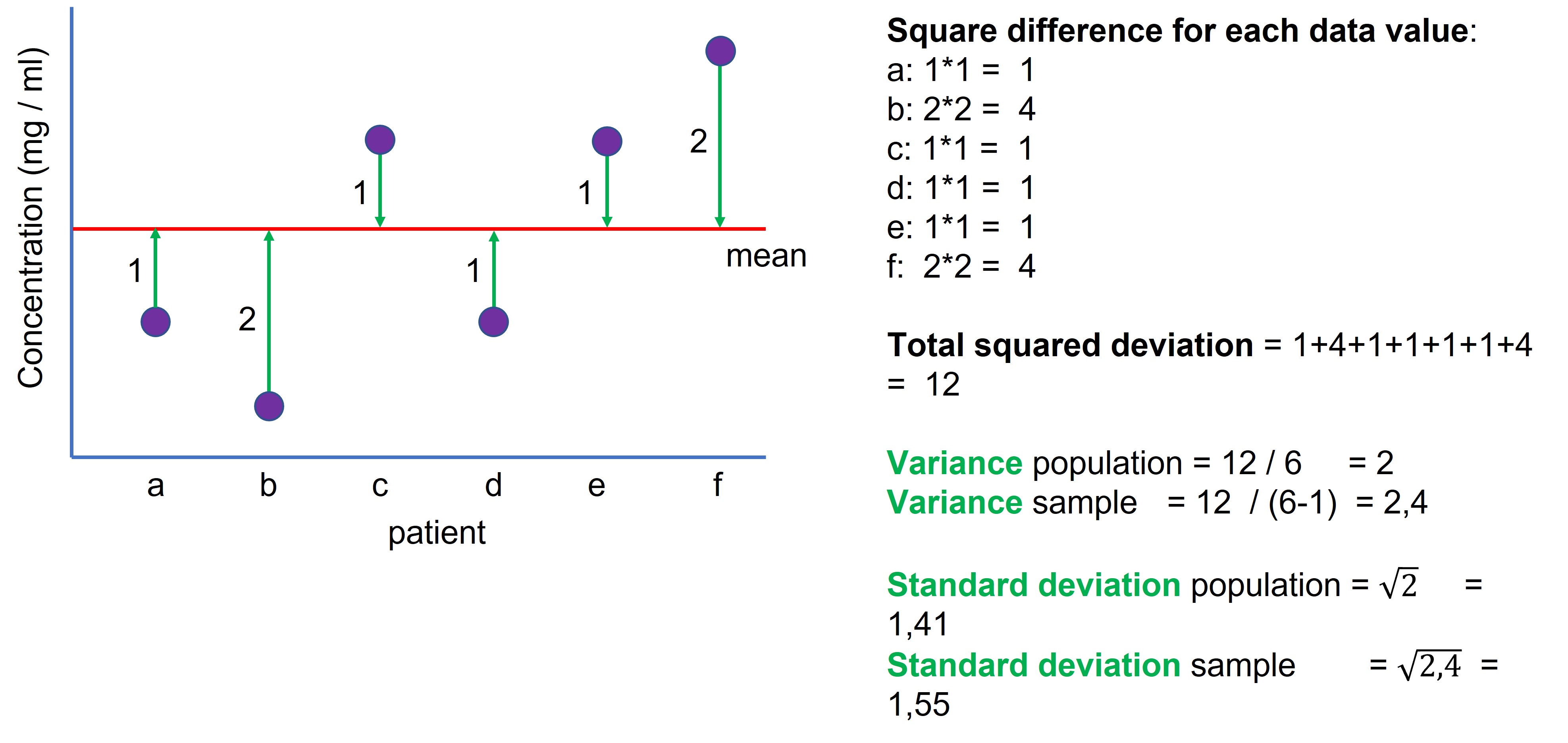
Figure 75: How to calculate the variance and the standard deviation

The symbol for the population variance: \(\sigma\)²
The symbol for the sample variance: s²

IMPORTANT: If the sample data is derived from a normal distribution, the mean summarizes the data with the least variance. In other words, the sample mean is the best estimate of the population mean.

IMPORTANT: Because the difference between the individual data points and the mean value are squared when calculating the variance (and the standard deviation, see below), any outlier will have a big impact on the value of these statistics (Figure 86).

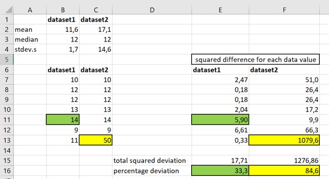
Figure 76: Outliers affect the variance

Data set 1 and 2 are identical except for the outlier in cell C13 (Figure 86)
The contribution of the highest value in data set1 (cell: B11) to the total squared deviation = 33,3% (cell: E16)
The contribution of the highest value in data set2 (cell: C13) to the total squared deviation = 84,6% (cell: F16)

Thus, a single outlier value is responsible for almost all of the deviation in data set2. It is therefore important to spot outliers in your data set. This outlier biases the total squared deviation -> variance -> standard deviation -> standard error of the mean (SEM) -> confidence intervals. Therefore, these statistics are not good estimates of the true population parameters.

lesson_09_assignment

A researcher obtains the following data points:

2, 3, 4, 5, 3, 4, 20

It is clear that 20 deviates from the other values.
Calculate the contribution (in % ) of value 20 to the total squared deviation (see also Figure 86)

Standard deviation

Standard deviation: square root (= worteltrekken) of the variance

The symbol for the population standard deviation: \(\sigma\)
The symbol for the sample standard deviation : s or s_n-1

The mean by itself doesn’t indicate how much variation is within a sample. Therefore the mean should always be written with the standard deviation. Reversely, the standard deviation is only meaningful relative to the mean. Consider the following example with two equal standard deviations:

sample 1: mean = 50, standard deviation = 10
sample 1: mean = 20, standard deviation = 10

In both cases the standard deviation is 10. But 10 relative to 50 is a less dramatic variance as compared to 10 relative to 20. Therefore, a useful way of expression deviation is the Coefficient of variation

Coefficient of variation (CoV)

CoV: standard deviation divided by the mean of the data set (multiplied by 100)

sample 1: mean = 50, standard deviation = 10, CoV = 10 / 50 = 20%
sample 1: mean = 20, standard deviation = 10, CoV = 10 / 20 = 50%

As a rule of thumb: a CoV < 10 is very good, between 10-20 is good and between 20-30 is acceptable.

Standard error of the mean (SEM)

SEM: standard deviation of a sampling distribution

The standard error is calculated using the standard deviation of the sample divided by the square root of n (= size of your sample)

SEM = s / sqrt(n)

We use the SEM to assess how accurately the sample mean represents the population mean using the concept of a sampling distribution:

A sampling distribution is a hypothetical concept in statistics. Let’s assume we want to study a population (for example, a group of diabetics patients with high blood pressure). From this population we want to know the mean concentration of a metabolite in the blood. On beforehand we know that this parameter has a value of 10. However, in reality we don’t know this value because it is impossible to measure all individuals of the population (but for know, by some magical intervention by a statistics fairy, we know this value).

In the real world, we estimate the true value of the population mean by taking a sample and calculate the sample mean (Figure 87, sample1: mean = 8). If we take another sample of the same size from the same population we would obtain yet another sample mean (sample2: mean = 9). If we repeat this process we will obtain different samples means (Figure 87, samples 2 t/m 9).

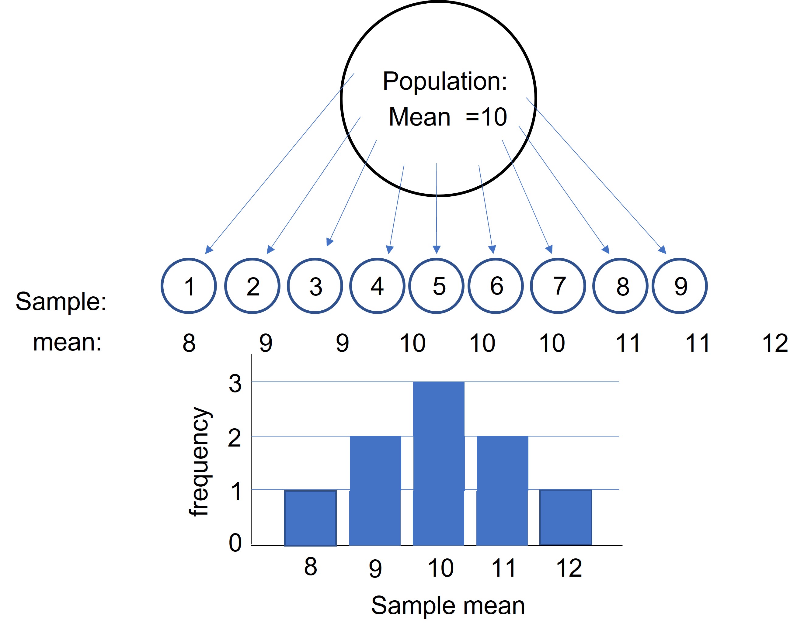
Figure 77: Sampling distribution

So, which sample mean is most representative for the population mean? If we make a distribution plot of all the different sample means (= sampling distribution) we will obtain a normal distribution and the value that occur most, will represent the population mean (Figure 87). The distribution of the sample means follows a normal distribution if the size of our samples is > 30. Using the normal distribution, we can calculate the lower and the upper limit of a 95% confidence interval: 95 of the 100 of the sample means will be within the limits of this interval. Sampling distributions are crucial because they place the value of your sample statistic into the broader context of many other possible sample values and indicate the variation between the sample means. This variation is called the standard error of the mean (SEM) and can be calculated by the standard deviation of the sample means (= between samples means and not within the individual samples)

In reality we won’t take many samples, make a distribution plot and calculate the mean and standard deviation of the sample means. We will only take one sample out of many possible samples! But how accurate will this sample represent the population mean. This depends on how much variation is present between the sample means. If the values of the sample means are more spread out, then a single sample mean will be more inaccurate to represent the true population mean compared to values of sample means which are close to each other (= less variation between the samples means). This variation between sample means (SEM) can be estimated from the standard deviation of a single sample ( SEM = s / sqrt(n))

Using the SEM we can construct confidence intervals around the mean of a single sample to indicate that the population mean lies somewhere within this interval:

lower limit: x̄-1,96*SEM
upper limit: x+1,96*SEM

If we use a confidence of 95% , this means that if we take 20 samples, calculate the mean, standard deviation and the corresponding confidence interval, for 19 samples the confidence interval will contain the true population mean (Figure 88). Or to put it the other way around, for 1 out of 20 samples the confidence interval will not contain the true population mean (Figure 88, green confidence interval)

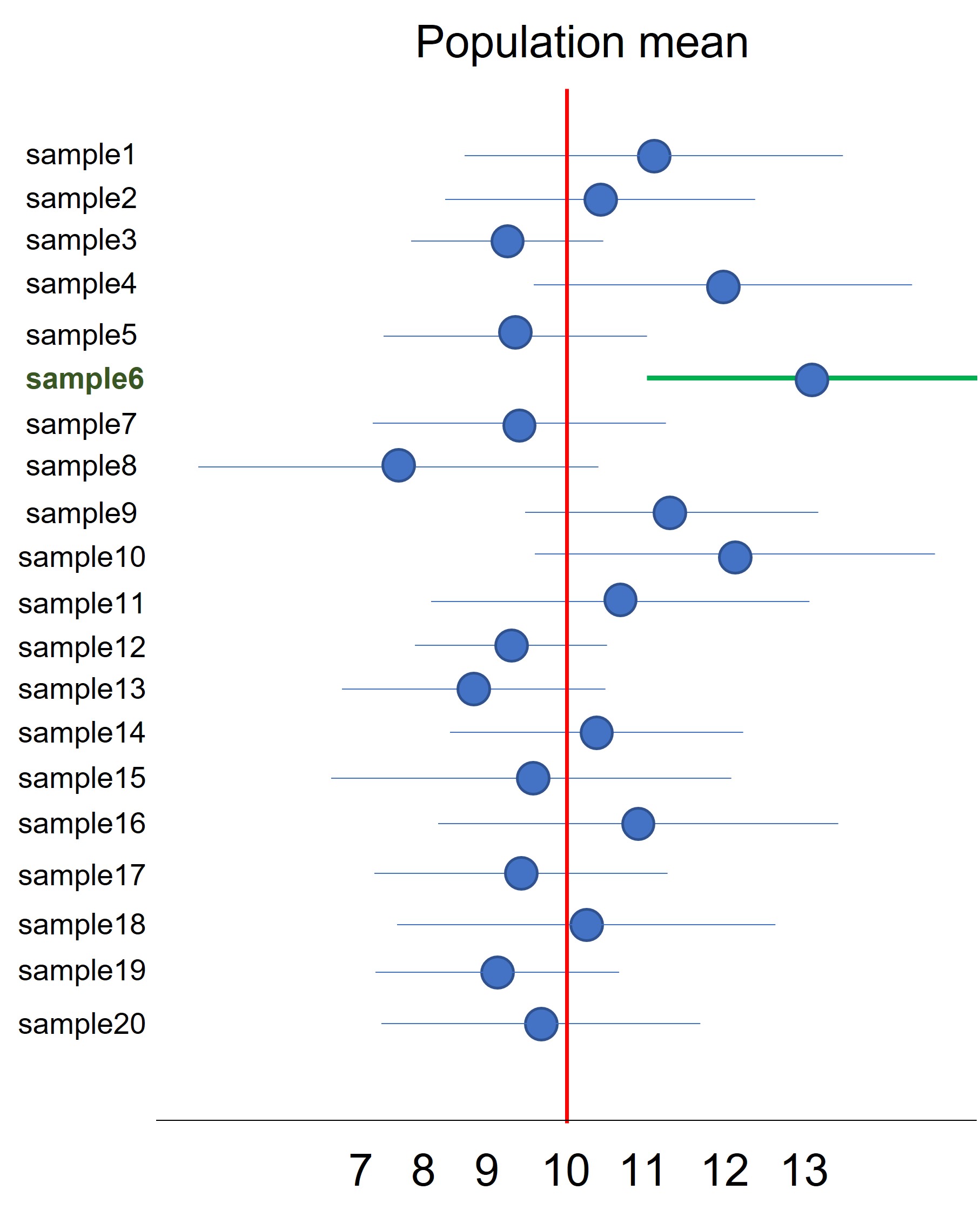
Figure 78: Confidence intervals

The problem with this approach is that on beforehand you will never know if your sample and corresponding confidence is one of the 19 that do contain the true population mean or the one that do not contain the true population mean. With this approach you’re taking a long term risk that in 1 out of 20 experiments your conclusion is wrong (more about type I and type II errors later). To understand the concept of long term probability think about leaping over an abyss. On beforehand, they will tell you there is a 75% chance of leaping over the abyss and survive. But, if you make the jump you don’t have a 75% chance of surviving. You either survive (100%) or fall in the abyss (0%) !! The long-term chance is calculated based on many people that leaped over the abyss.

REMINDER:
- standard deviation: deviation of the individual values within a sample relative to mean of the sample
- standard error of the mean (SEM): deviation between the sample means of a sampling distribution

Inferential statistics

Parametric test are related tests which are used to statistically test if a difference between a sample mean and a population mean (one sample t-test) or between the mean of samples (two-sample t-test, ANOVA) is significant.

There are three variants of parametric tests:

One sample t-test
Two sample t-test

paired
unpaired

ANOVA (more than three samples)

one way
two way

A parametric test may only be used if all three of the following conditions are met:

Comparative research question
Quantitative data
Sample data is a good estimate of the population mean (no outliers present in the data set)
The sample data is normally distributed

The first two requirements are determined by your experimental set-up. The other requirements will be explained below

Spotting outliers

Before performing a parametric test we have to be sure that our sample mean represents the population mean. We have learned that an outlier has a strong influence on the mean and variance (and derived from the variance -> standard deviation -> SEM -> confidence intervals). If these statistics are biased from the start (meaning that they do not represent the population parameters) there is no use in performing parametric tests.

Outliers can be generated by:
- An “avoidable mistake”: for example the value is 2,02 and accidentally you noted 20,02
- Natural variation within your sample
- Bad practice in the lab: for example miscalculation, or bad pipeting

The best way to spot outliers is to calculate the Coefficient of Variation in combination with visualization of the data:
- Distribution plots
- Boxplots
- Dot plots

lesson_09_assignment

Copy data file lesson_09_opdracht4.txt from the shared directory to your home directory -> lesson_09
Import the data files in JASP
Create a distribution plot, boxplot and a dot plot

What is the value of the outlier?

Removing outliers

If your sample contains an outlier, the sample mean is not a good estimate of the population mean. Therefore, we have to remove the outlier.

There are several test and techniques to remove an outlier:

Dixon’s Q test to spot an outlier: this test is limited to repeated measurements and can only be used once to spot an outlier in the data
Another method is to remove any data value that is > 2,5 standard deviations from the mean
Data trimming: remove lowest and highest data values

Always include the raw data and describe the method that has been used to remove the outlier!

Although we remove outliers from the sample, an outlier by itself could be an interesting observation worth further investigation. Perhaps you have discovered the exception to the rule!!

First we use the method of 2,5 standard deviation:

lesson_09_assignment

A researcher obtains the following data points:

2, 3, 4, 5, 3, 4, 20

Can we remove the value 20 based on the method that a value > 2,5 standard deviations from the mean?
What is your conclusion?

A better method is trimming the data: removing a certain percentage of the lowest and highest scores (Figure 89)

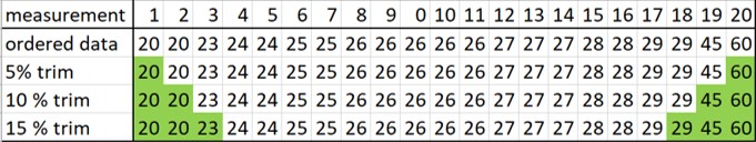
Figure 79: Data trimming

lesson_09_assignment

Copy data file lesson_09_opdracht6.txt from the shared directory to your home directory -> lesson_09

This data file contains the data of Figure 89. Remove the values which are marked in Figure 89 to trim the data

Calculate for the original and the trimmed data the mean, median and standard deviation
Make one single boxplot of the original and the trimmed data
What is the effect of data trimming on the mean, median, standard deviation?

Spotting normality

The other requirement for performing parametric tests is that the values in the sample are normally distributed (formally, it means that the residuals, the difference between a single value and the sample mean (see Figure 85, green arrows), are normally distributed). In other words, if the data is normally distributed, the mean is the best single point estimate with the least variance.

IMPORTANT: Testing normality is important is you have sample sizes < 30. If your sample is > 30 the central limit theorem (CLT) states that the distribution of sample means approximates a normal distribution. However, this depends on how much the population is skewed. If the population is slightly skewed then a size of 30 is sufficient. If the data is heavily skewed then bigger samples are required for the CLT to hold. The best practice is to always check for normality with distribution plots, q-q plots and the Shapiro-Wilk test.

To test if your data in your sample (n < 30) is normally distributed we can:

Visualize the data using

distribution plots: look for a symmetrical bell shape (with n < 30, this could be hard to spot)
dot plots: look for a symmetrical distribution
q-q plots: values (dots) in the q-q plot should be close to the straight line

Calculate sample statistics to assess normality

Skewness: value for the skewness should be close to zero. Between -1 and 1 is accepted as close enough to normality
kurtosis: value for the kurtosis should be close to zero. Between -1 and 1 is accepted as close enough to normality

Perform the Shapiro-Wilk test: p-value > 0,05 indicates normality

To conclude that our data approximates a normal distribution we have to consider all the different methods as stated above. Never conclude that your sample data is normally distributed based on only a single figure, statistic or test!

lesson_09_assignment

Copy data file lesson_09_opdracht7.txt from the shared directory to your home directory -> lesson_09
Open the file in JASP
For each group:
- calculate the default statistics + Skewness, Kurtois and perform the Shapiro-Wilk test
- Basic plots: Distribution, Q-Q and Dot plots

Combine these analyses and for each group conclude whether the data is normally distributed or not.

Parametric tests

If your sample values are free of outliers and are normally distributed we can perform parametric test. These tests use the sample mean as estimate of the population parameter. If the data is not normally distributed we will have to use alternative methods which will be described in lesson_10

Here, we will briefly introduce the one-sample and two-sample T-test and how to perform them in JASP.

One Sample T-test

The “One sample T-test” compares a sample mean to a given population mean. The research question is whether a sample is derived from a population of which the mean is known. First formulate the null (H₀) and the alternative (H₁) hypothesis:

H₀: There is no difference in “what has been measured” between the sample mean and the provided population mean
H₁: There is difference in “what has been measured” between the sample mean and the provided population mean

IMPORTANT: In parametric testing the H₀ hypothesis always state that there is no differences between the sample means.

NOTE: In JASP we only define the H₁ which could be two-sided or one-sided. Always choose the two-sided option unless you have good scientific arguments to choose the one-sided option. The one-sided option is less stringent and you will obtain more easily a p-value < 0,05 and thus conclude that the treatment has worked. If you don’t have a good reason to use a one-side test it will be p-hacking

The One sample T-test first calculates the difference between the population mean and the sample mean. This difference is divided by the SEM of the sample you want to test. This value is the t-statistics and is a measurement of “how far” the sample mean is from the population mean. A large t-statistic indicates a big difference between the sample mean and the population mean and results in a small p-value (which is the chance of observing such a difference under the assumption of the H₀: there is no difference).

If the p-value > 0,05: accept the H₀
If the p-value < 0,05: reject the H₀ and accepts the H₁

To perform a “One sample T-test” select in the main menu of JASP -> T-Tests -> Classical -> One Sample T-Test
(To preform a “One sample T-test” on multiple samples in JASP, the data values for each sample should be listed in a separate column)

The file lesson_09_opdracht8.txt contains the creatine concentration as determined in the blood samples of 50 patients infected with hepatitis B. We wonder whether infection with hepatitis B can lead to an increased creatine concentration in the blood. We know that healthy people have a creatine concentration of 92 mol/l. So in this case there is only 1 sample that we want to compare with a known population value

lesson_09_assignment

Copy data file lesson_09_opdracht8.txt from the shared directory to your home directory -> lesson_09
Open the file in JASP
Perform descriptive statistics to test for outliers and normality

Does the data set contain outliers?
Is the data normally distributed?
Why don’t we have to test for normality?

Open the One sample T-test panel in JASP
Fill out the panel as shown in Figure 90:

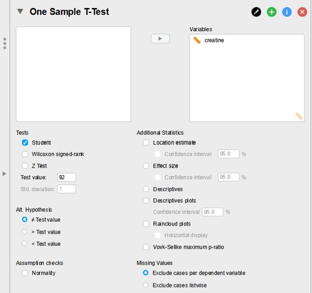
Figure 80: JASP: One sample T-test

Test value: 92 (this is the provided population mean)
Alt. Hypothesis: is non equal Test value
(The other options relate to one-side hypothesis testing)

The output of the one sample T-Test (Figure 91):

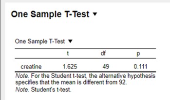
Figure 81: JASP: One sample T-test

t-statistic of 1,625
degree of freedom of 49 (= n-1 = 50-1 = 49)
p-value of 0,111

The p-value is > 0,05 and therefore we accept the H₀. The difference we have observed between the sample mean and population mean is just by chance and therefore not statistically significant. The difference can be explained by random sampling variation and falls within the 95% confidence interval of the population mean (is close enough to the value of 92)

lesson_09_assignment

A nephrologist conducts research on two groups of patients, each with a different kidney disease. She wants to know whether the kidney disease can be linked to a decreased concentration of a metabolite in the urine of the patients. The population mean of the metabolite concentration of healthy persons is 105 mg / ml

Copy data file lesson_09_opdracht9.txt from the shared directory to your home directory -> lesson_09
Open the file in JASP
Perform descriptive statistics to test for outliers and normality

Is the data for each group normally distributed?
Does the data contain outliers?
Does the sample mean of group1 and group2 come from a population with a mean of 105 mg / ml?
What is your conclusion?

Independent Samples T-test

A classic experimental design is to compare the means of two independent samples. Two independent samples are drawn from a population:

Sample 1: control group (also called the reference groups or baseline group)
Sample 2: treatment group

Before we do the Independent Samples T-test let’s think what will happen if we randomly draw two samples from the same population without any treatment. The samples have the same characteristics and therefore these samples should have more or less the same mean value for “what has been measured” ( = outcome variable). However, we know from the sampling distribution that sample means from the same population differ by chance alone. Thus, without any treatment we already expect a difference between sample1 and sample2 and this difference should be most of the time close to zero. However, by chance alone, we could also draw two samples from the same population of which the difference in means is quite far from the expected zero, although this happens less frequently. The bigger the difference between sample means (from the same population), the less frequent this will occur by chance alone. How often this will occur can be visualized and calculated using a sampling distribution:

A thousand times, we draw two samples from the population, calculate the mean for each sample and the difference between them (Figure 92, as an example we draw 9 pairs of samples). From these values we create a distribution plot (Figure 92, the distribution plot is based on 2686 pairs of samples). This distribution follows a normal distribution so we can calculate a 95% confidence interval. Thus, the values between the lower and upper limits of the confidence interval are the differences between two random samples which is expect by chance alone, before the start of the treatment!

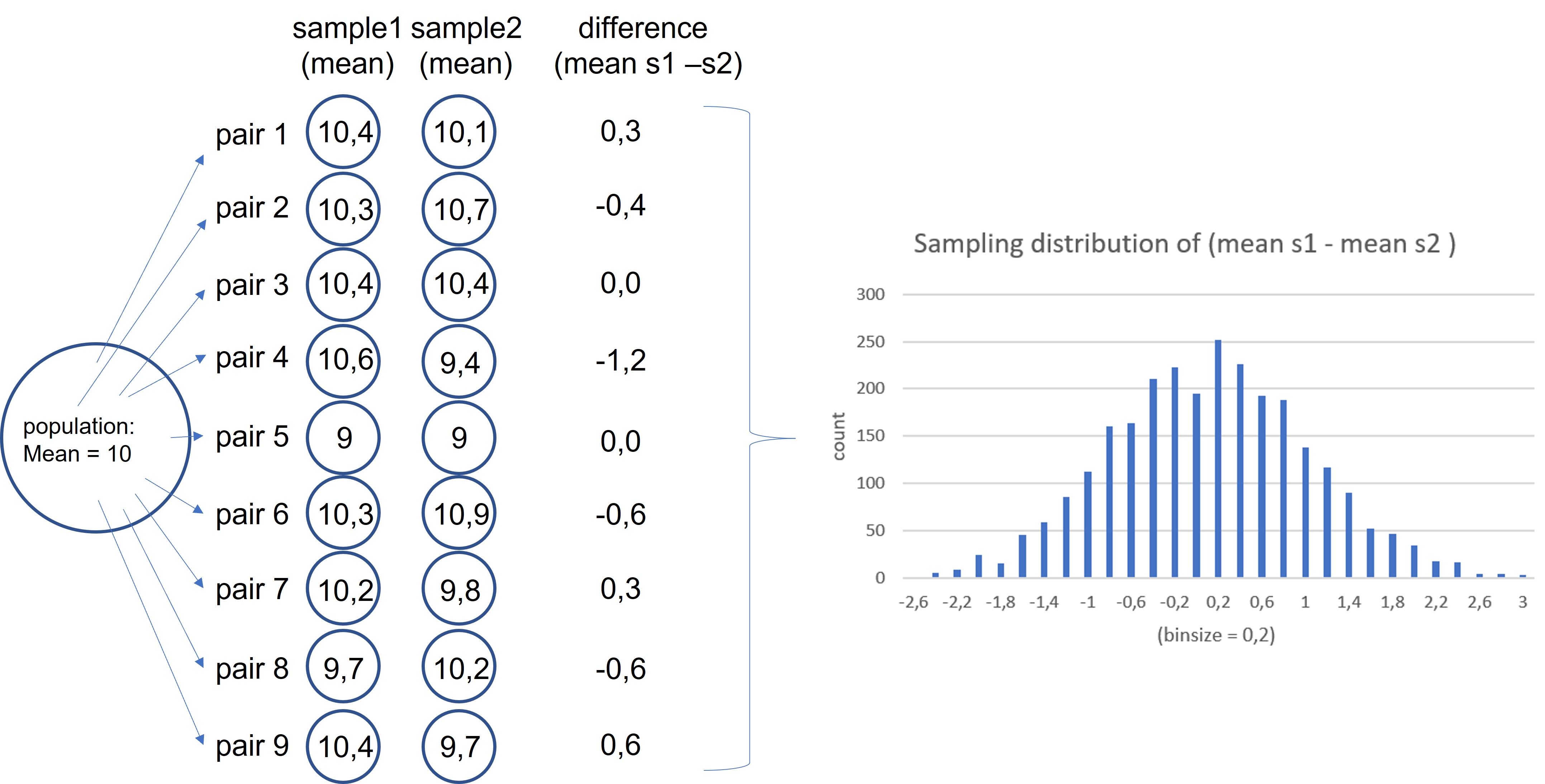
Figure 82: JASP: Sampling distribution of the difference between two sampole means

In the experimental set-up we treat one sample as a control (= reference or baseline sample) and the other sample receives the treatment. If the treatment is not working we expect the sample means to be more or less equal and the difference between them lies within the 95% confidence interval. We conclude that any difference we observe is caused by chance alone. If the treatment works, the difference between control and treated sample has to be outside the 95% confidence interval to call it statistical significant. We conclude that the difference between the control group and the treatment group can’t be explained by chance alone, but that the treatment also has contributed to this difference. The treatment has worked.

To address the research question whether the treatment has an effect, we have to formulate the null (H₀) and the alternative (H₁) hypothesis for the Independent samples T-test.

H₀: There is no difference in the mean value of “what has been measured” between sample1 and sample2 (the means are equal)
H₁: There is difference in the mean value of “what has been measured” between sample1 and sample2 (the means are unequal)

The first step in the “Independent samples T-test” is to calculate the difference between the sample means of the control group and the treatment group. This difference is divided by the combined SEM of sample 1 and 2. This value is the t-statistics and is a measurement of “how far” this difference is from 0. A large t-statistic indicates a big difference (far from 0) and results in a small p-value (which is the chance of observing such a difference under the assumption of the H₀: there is no difference).

If the p-value > 0,05: accept the H₀
If the p-value < 0,05: reject the H₀ and accepts the H₁

To perform an “Independent Samples T-test” select in the main menu of JASP -> T-Tests -> Classical -> Independent Samples T-test

When performing the Independent Samples T-test we have to organize the data in two columns. One column contains the data and the second column list the group to which the data belongs:

If we have the following dataset:

sample1 (control) : 10, 12, 11, 14, 12
sample2 (treatment): 13, 15, 14, 13, 16

It should be organized in two columns:

data	group
10	1
12	1
11	1
14	1
12	1
13	2
15	2
14	2
13	2
16	2

Before doing an independent samples T-test we have to check:
1. if the data contains outliers
2. if both samples are normally distributed

For the “Independent Samples T-test” we also have to check for equality of variance

The assumption equal of variance is only relevant for samples < 30, different sample sizes or both. When performing the “Independent samples T-test” go to “Assumptions Checks” and check “Equality of variances”. In the output screen, a panel will show “Assumption Checks” -> Test of Equality of Variance (Levene’s). If p-value > 0,05 the variances are equal. If the p-value < 0,05 we will have to apply a Welch correction which result in a more conservative p-value. The Welch correction can be found at Tests -> Welch

lesson_09_assignment

An oncologist wants to measure the size of colorectal cancer after treatment with a new bio-pharmaceutical. The oncologist selected patients with a stage I tumor with tumor sizes of less then 2 cm. The patients were divided into two groups:

group1: control without treatment
group2: treatment with new bio-pharmaceutical

Copy data file lesson_09_opdracht10.txt from the shared directory to your home directory -> lesson_09
Open the file in JASP
Perform descriptive statistics to test for outliers and normality

Is the data for each group normally distributed?
Does the data contain outliers?
What is the p-value of the Levene’s test. Do the samples have equal variance?
Is there a statistical significant difference in tumor size between the sample means of group1 and group2? (Don’t forget to define the H₁)
What is your conclusion?

Paired Samples T-test

A paired Samples T-Test is used if your experimental design includes one group which is measured twice thus generating two related ( = paired ) samples. A common variant (but not the only variant) of a paired experimental design is a measurement before the treatment and a measurement after the treatment for each subject in the group. The advantage of this design is that each subject in the group serves as its own control and this reduces random differences between the measurements. Therefore, a paired experimental design has more power to detect differences which are caused by the treatment, because the differences that occur by chance are reduced. However, it is not always possible to have a paired experimental set-up, for example when you have to sacrifice your modelsystem to collect tissues, DNA, RNA, proteins and so on.

To address the research question whether the treatment has an effect, we have to formulate the null (H₀) and the alternative (H₁) hypothesis for the Paired Samples T-test.

H₀: There is no difference in the mean value of “what has been measured” between the before and after samples (the means are equal)
H₁: There is difference in the mean value of “what has been measured” between the before and after samples (the means are unequal)

The first step in the “Paired samples T-test” is to calculate, for each entity in the sample, the difference between the before and after values. Thus, from two samples a single sample is generated. From this new sample we calculate the mean and the SEM. If there is no effect of the treatment the mean value of the differences should be around 0. The mean value of the differences is divided by the SEM. This value is the t-statistics and is a measurement of “how far” the mean difference is from 0. A large t-statistic indicates a big difference (far from 0) and results in a small p-value (which is the chance of observing such a difference under the assumption of the H₀: there is no difference).

If the p-value > 0,05: accept the H₀
If the p-value < 0,05: reject the H₀ and accepts the H₁

To perform a “Paired Samples T-test” select in the main menu of JASP -> T-Tests -> Classical -> Paired Samples T-test

When performing a Paired samples T-test we have to organize the data in two columns. The first column contains the “before” data and the second column contains the “after” data:

If we have the following dataset:

sample1 (before): 10, 12, 11, 14, 12
sample1 (after) : 13, 15, 14, 13, 16

It should be organized in two columns as shown below:

before	after
10	13
12	15
11	14
14	13
12	16

Before doing a paired samples T-test we have to check:
1. if the data contains outliers
2. if the difference between the paired samples is normally distributed:

NOTE: we don’t have to check for “Equal of variance” because we end up with only one sample ( = difference between the paired samples )

lesson_09_assignment

A nephrologist wants to test whether administrating EPO to patients with kidney failure affects hematocrit levels. EPO is a hormone produced in the kidneys and regulates the production of red blood cells. A group of patients is measured for hematocrit levels before and after the treatment.

Copy data file lesson_09_opdracht11.txt from the shared directory to your home directory -> lesson_09
Open the file in JASP
Perform descriptive statistics to test for outliers and normality

Is the data for each group normally distributed?
Does the data contain outliers?
Is there a statistical significant difference in hematocrit levels between the sample means of group1 and group2? (Don’t forget to define the H₁)
What is your conclusion?