Lesson_10 - Statistics Part2

Learning objectives

The student is able:

To perform ANOVA analysis in JASP
To perform correlation analysis in JASP
To perform regression analysis in JASP
To perform non-parametric tests in JASP

Introduction

In the previous lesson we have learned how to perform parametric tests to compare two sample means. In this lesson we will discuss Analysis of Variance (ANOVA) to compare three or more groups in JASP. In addition, we will repeat and extend our knowledge about correlation and regression analyses and lastly what to do when the data is not normally distributed?

One way ANOVA

There are two variants of a One way ANOVA (Figure 93):
- independent
- paired

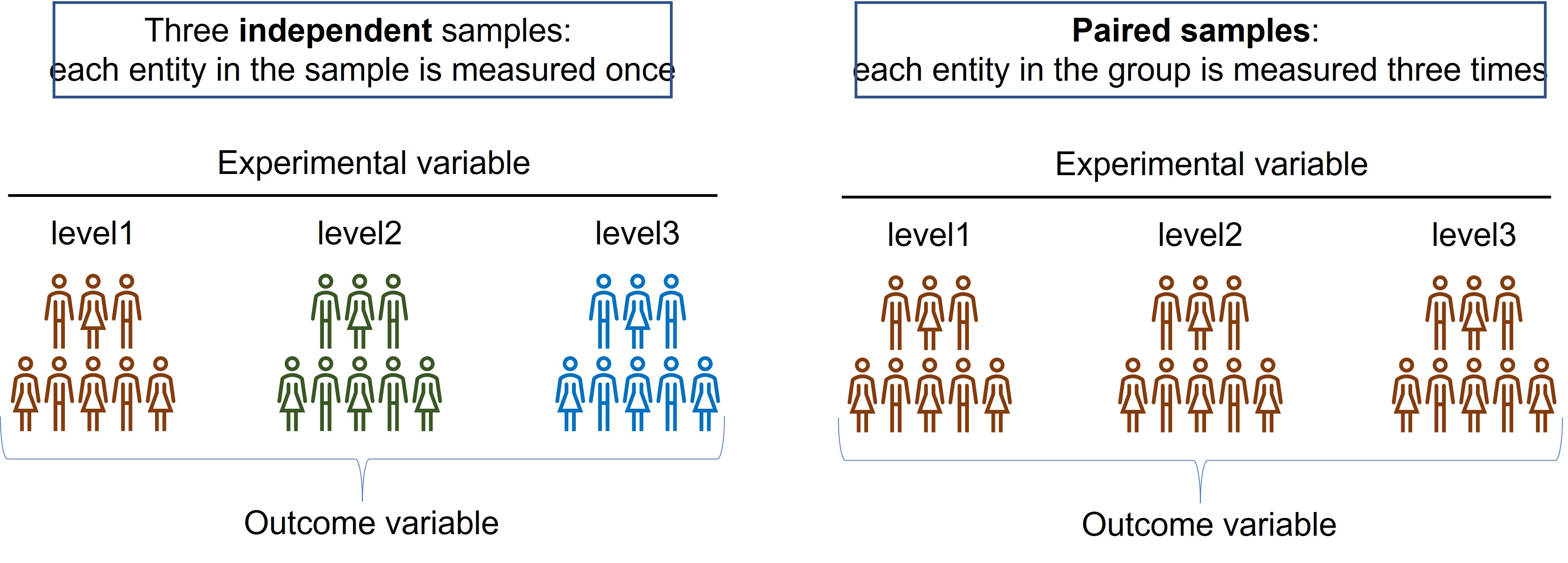
Figure 83: One way ANOVA

In an independent samples design, each group receives a so called level of the experimental variable. For example, each group receives a different concentrations of a chemical or different exposure time of a treatment. Level1 is most often the control ( = baseline or reference group) and don’t receive the treatment or is the starting point in a time series.

In the paired design each entity in the group receives the three levels of the treatment and is measured after each treatment

ANOVA for independent samples

A cancer researcher wants to test whether the addition of a mono clonal antibody in two concentrations inhibits cell signalling in cancer cells:

mono clonal antibody (= experimental variable) -> cancer cell line (= model system) -> inhibition of signalling pathway ( = outcome variable)

Sample 1: control group (without treatment, also called the reference groups or baseline group) Sample 2: mono clonal antibody concentration 1 Sample 3: mono clonal antibody concentration 2

Here, we have two hypothesis: We predict that treatment of the cancer cells with the mono clonal antibodies has an effect on the signalling pathway and in addition we predict that this effect is concentration dependent.

To address the research question whether the treatment has an effect we have to formulate the null (H₀) and the alternative (H₁) hypothesis for ANOVA

H₀: There is no difference in the mean value of “what has been measured” between the samples (the sample means are equal)
H₁: There is difference in the mean value of “what has been measured” between the samples (the sample means are unequal)

Before we do the ANOVA, let’s think what will happen if we randomly select three independent samples from the same population. The samples have the same characteristics and therefore these samples should have more or less the same mean value for “what has been measured” ( = variable). If the treatment is not working ( = H₀ ) each sample represents the population mean and thus we can calculate the mean based on all values combined from the three samples (Figure 94, dotted red line: grand mean).

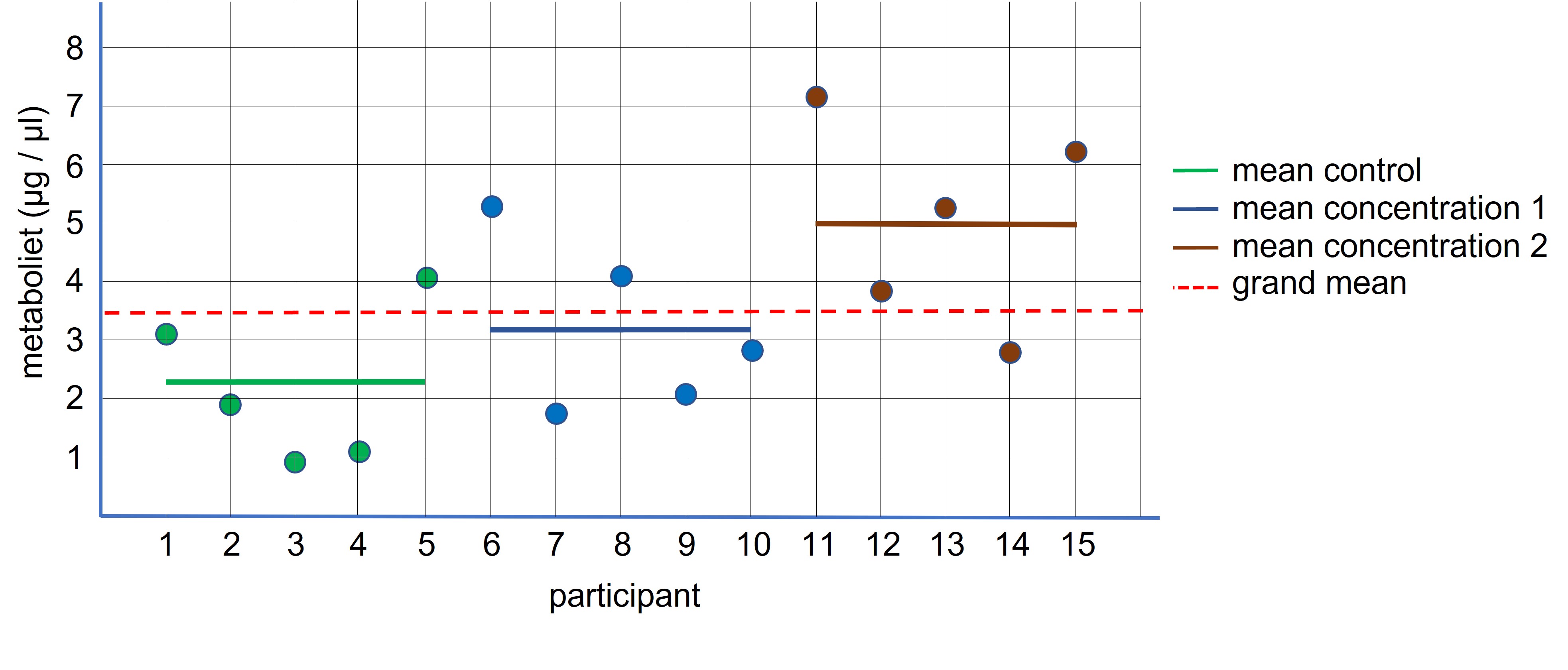
Figure 84: ANOVA: independent design

If the means of the three samples are equal we don’t expect a lot of deviation relative to the grand mean (because the grand mean is calculated based on the sample means and the sample means and the grand mean should be more or less be equal). If there is a substantial difference between the individual sample means and the grand mean it is more likely that the sample means differ from each other and that the manipulation has worked (contributed to the difference sample means).

The first step in an ANOVA analysis is to calculate the difference between the sample means and the grand means (Figure 95, difference between the straight colored lines and the dotted red line). This difference is multiplied by the number of entities in the sample (because each entity in the sample has contributed to the sample mean) and the three group differences are added together to calculate the difference between the samples. (We also divide this value by the number of degrees which is the number of groups -1 = 3 -1 = 2)

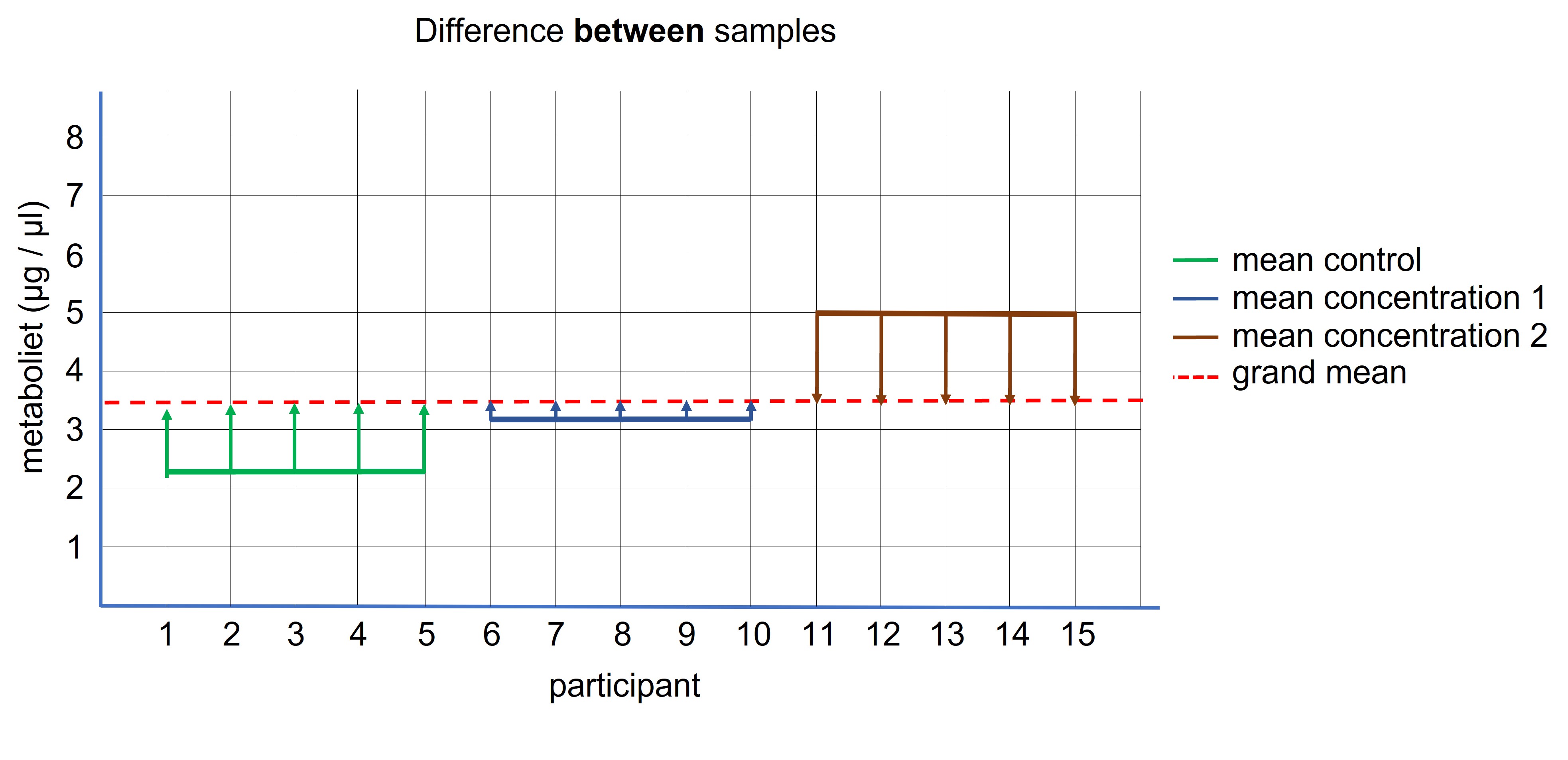
Figure 85: ANOVA: difference between the samples

The second step is to calculate the difference within the samples, because this is the difference we expect by chance (Figure 96). These differences are also added together to calculate the total difference within the samples and serves as our noise ( = difference we expect by chance only). (We also divide this value by the degree of freedom which is the total number of (entities) -1 = (3 * 5) -1 = 15 -1 = 14 )

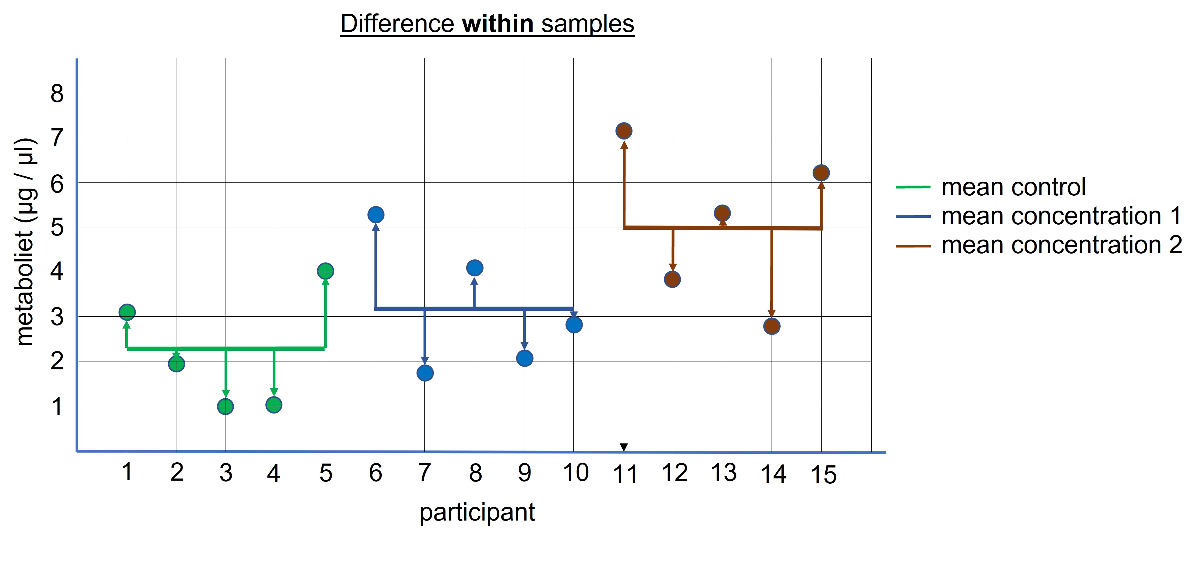
Figure 86: ANOVA: difference within the samples

Next, we calculate the F statistics which is the (differences between the samples) / (differences within the samples). In other words the signal we expect from the treatment divided by the noise (random differences) from the experiment. The bigger this F-statistic, the more likely that the difference between sample means is not because of random chance but due to the treatment.

If the chance ( = p-value) > 0,05: accept the H₀
If the chance ( = p-value) < 0,05: reject the H₀ and accepts the H₁

IMPORTANT:ANOVA tests if there is a difference between the groups but the output doesn’t indicate which groups differ. But what is the point of doing an ANOVA if we can only say that there is a difference somewhere between the groups!! Can’t we do independent Samples T -test between sample1-sample2, sample1-sample3 and sample2-sample3? The answer is NO.

Using the procedure of null hypothesis testing we use a p-value of 0,05 as our threshold. If we observe a difference between sample means that is large, so that the chance of obtaining such a difference by chance alone is smaller then 5% (under the assumption that there was no difference to start with) we called it a statistical significant difference between the sample means. But this difference could still be explained by chance alone although this chance is less then 5%. Thus, this threshold means that we accept a 5% chance ( 1 out of 20 comparisons) of making a so called type I error ( = false positive): we state that there is statistical difference, but in reality the observed difference is due to chance.

To calculate the type I error for multiple testing (= family wise error rate) we use the following formula: 1 - (1 - significance threshold)^number of comparisons^ *100

1 test: 1 - (1 - 0,05)¹ * 100 = 5 %
2 tests: 1 - (1 - 0,05)² * 100 = 9,75 %
3 tests: 1 - (1 - 0,05)³ * 100 = 14,3 %

Thus, with three comparisons we increase the chance of making a type I error ( = false positive) from 5% to 14,3 %

To correct for this increase we can first perform an ANOVA, to check if there is a difference between the groups. If so, we continue with post-hoc analyses. This analysis performs the pair-wise comparison between the groups but corrects for the type I error rate and keeps the total error rate at 5%. There are several post-hoc tests of which the Bonferroni and Tukey correction are most frequently used.

lesson_10_assignment

A researcher wants to test gene expression levels in liver cells which were exposed to PFAS. The researcher obtained for 20.000 genes expression values for the control group and the treated group. The researcher performs 10 independent samples T-tests.

Calculate the type I error for multiple testing if the researcher performs 10 independent samples T-tests

Before doing an ANOVA analysis for independent samples we have to check:

The level of measurement is quantitative
No presence of outliers
Data is normally distributed

For ANOVA we also have to check for equality of variance between samples

The assumption equal of variance is only relevant for samples < 30, different sample sizes or both. When performing ANOVA go to “Assumptions Checks” and check “Homogeneity tests. In the output screen, a panel will show”Assumption Checks” -> Test of Equality of Variance (Levene’s). If p-value > 0,05 the variances are equal. If the p-value < 0,05 we will have to apply a Welch correction which result in a more conservative p-value. The Welch correction can be found at the “Assumption Checks” -> Homogeneity corrections -> Welch

IMPORTANT: When performing the ANOVA for independent samples we have to organize the data in two columns. One column contains the data and the second column list the group to which the data belongs

lesson_10_assignment

A nephrologist wants to test whether administrating different concentrations of EPO to patients with kidney failure affects hematocrit levels. EPO is a hormone produced in the kidneys and regulates the production of red blood cells.

group1: no treatment
group2: EPO concentration 1
group3: EPO concentration 2

Copy data file lesson_10_opdracht2.txt from the shared directory to your home directory -> lesson_10
Open the file in JASP
Perform descriptive statistics to test for outliers and normality

Is the data for each group normally distributed?
Does the data contain outliers?
Do the samples have equal variances?

To perform a “ANOVA test” select in the main menu of JASP -> ANOVA -> Classical -> ANOVA

Next, check the following option:

Dependent Variable (= what has been measured) = hematocrit
Fixed Factors ( = groups )
Post Hoc Tests: Bonferroni

NOTE: We don’t have to check the H₀ and H₁ because ANOVA tests two-sided. ANOVA only tests whether there is a difference (and not the direction of the differences)

lesson_10_assignment

What is the p-value of the ANOVA test?
What is your conclusion?
What are the p-values of the pair-wise post-hoc tests?
What is your conclusion?

lesson_10_assignment

The nephrologist wants to test whether administrating two different types of EPO to patients with kidney failure affects hematocrit levels.

sample1: no treatment
sample2: EPO type 1
sample3: EPO type 2

Copy data file lesson_10_opdracht4.txt from the shared directory to your home directory -> lesson_10
Open the file in JASP
Perform descriptive statistics to test for outliers and normality

Is the data for each group normally distributed?
Does the data contain outliers?
Do the samples have equal variances?
What is the p-value of the ANOVA test?
What is your conclusion?
What are the p-values of the pair-wise post-hoc tests?
What is your conclusion?

Paired ANOVA

If there are three or more measurements of the same group we use an ANOVA for paired samples to test for differences between the sample means ( = levels) (Figure 97).

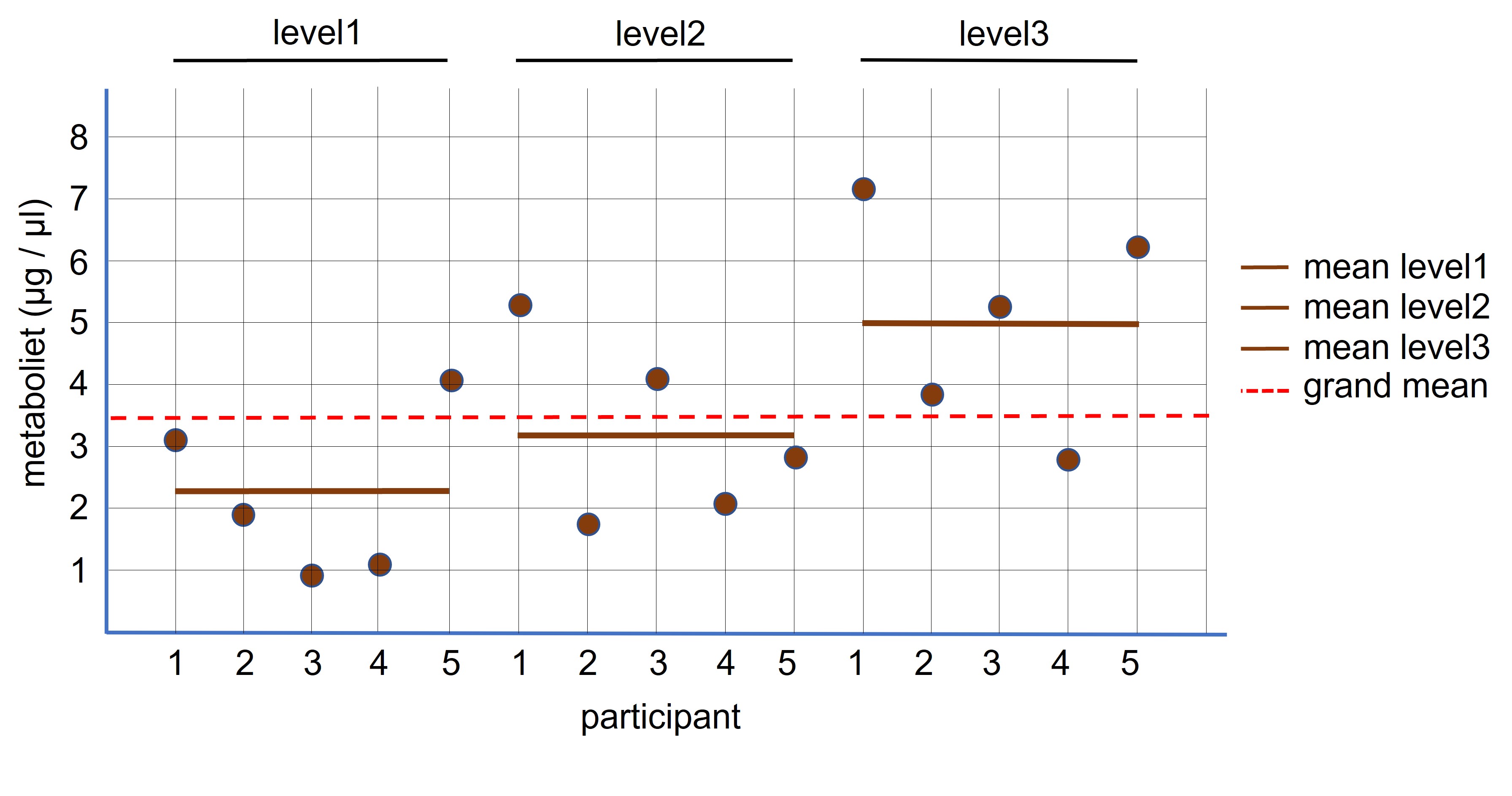
Figure 87: ANOVA: paired design

For example, patients underwent an exercise schedule to lower chronic inflammation. The patients were measured for the presence of a protein in their blood, which serves as a marker for inflammation, before and after the different times of the exercise program:

time1: before the start of the exercises
time2: after 4 weeks (time2)
time3: after 8 weeks (time3).

Here, we have two hypothesis: We predict that exercises has an effect on the protein concentration and in addition we predict that this effect is time dependent.

Table I: Repeated experimental design:

patient	time1	time2	time3
1	55	48	52
2	45	54	51
3	47	45	48
4	51	42	39
5	54	47	48

To address the research question whether the treatment has an effect we have to formulate the null (H₀) and the alternative (H₁) hypothesis for ANOVA

H₀: There is no difference in the mean value of “what has been measured” between the levels (the means are equal)
H₁: There is difference in the mean value of “what has been measured” between the levels (the means are unequal)

The ANOVA analysis for paired samples follows the same logic as described above for an ANOVA for independent samples:

If the exercises don’t have an effect on the protein concentration, the different levels (time1, time2 and time3) should have more or less the same mean value and thus we can calculate the mean value based on all values combined from the three levels ( = grand mean, see Figure 98).

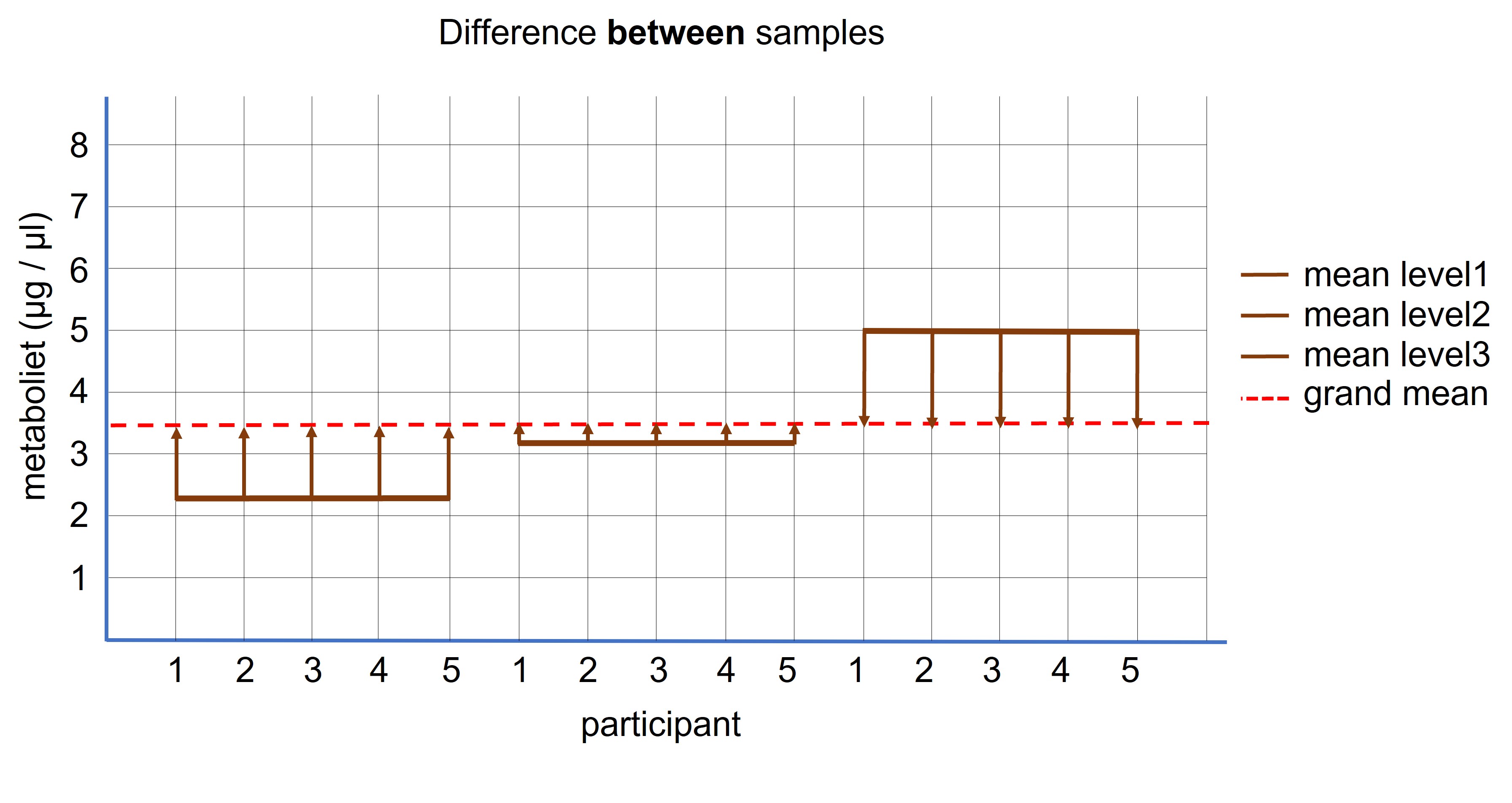
Figure 88: Paired ANOVA: difference between the samples

If the means of the three levels are equal we don’t expect a lot of deviation relative to the grand mean (because they are all from the same population). If there is a substantial difference between the mean of each level relative to the grand mean, it is more likely that the manipulation has worked (contributed to the different mean values of each level) (Figure 98).

The next step is to calculate the noise in the experiment which is how much of the different mean value of each level can be explained by chance alone. This calculations differs from the ANOVA of the independent samples (and will not be explained in detail here). Because it is a repeated experimental design, each participant serves as its own control and therefore the random noise in the experiment will be reduced. Therefore, a paired experimental design has more power to detect differences which are caused by the treatment, because the differences that occur by chance are reduced.

Next, we calculate the F statistics which is equal to the signal we expect from the levels ( = treatment ) divided by the noise (differences by chance) from the experiment. The bigger this F-statistic, the more likely that the different mean values of each levels can’t be explained by random chance but is due to the treatment.

If the chance (= p-value) > 0,05: accept the H₀
If the chance ( = p-value) < 0,05: reject the H₀ and accepts the H₁

Before doing an ANOVA analysis for paired samples we have to check:
1. if the data contains outliers
2. if the samples are normally distributed
3. Assumption of sphericity: are the variances of the differences between levels equal - First calculate the difference between time1-time2, time1-time3 and time2-3. - From these differences calculate the variance. - The variances should be more or less equal

Table II: Assumption of sphericity

patient	time1	time2	time3	time1-time2	time1-time3	time2-time3
1	55	48	52	7	-3	4
2	45	54	51	-9	6	-3
3	47	45	48	2	1	3
4	51	42	39	9	-12	-3
5	54	47	48	7	-6	1
			variance	53,2	46,7	10,8

(Don’t worry we can easily check this in JASP)

IMPORTANT: When performing an ANOVA for paired samples we have to organize each group in a separate columns:
level1 -> column 1
level2 -> column 2
level3 -> column 3

JASP contains a lot of in-built examples on how to perform a certain test:

Go to -> Open -> Data library -> 3. ANOVA (Figure 99)
Open the data of the Bush_tucker_food example

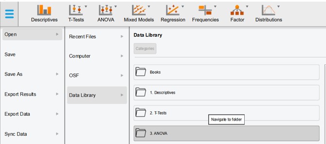
Figure 89: JASP: Data library

This data set is an example of an ANOVA analysis for paired samples

Study how the data is organised (Figure 100)

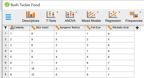
Figure 90: Paired ANOVA: data organization

Read the text describing the experimental set-up
Study how the test was executed (Figure 101)

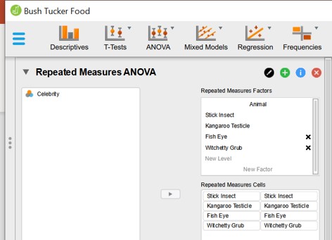
Figure 91: Paired ANOVA: repeated measures panel

In the Repeated Measures Factors the experimental variable is defined (animal) and the levels of this variable (Stick Insect, Kangaroo Testicle, Fish Eye, Witchetty Grub). This has to be entered by the user as text.
In the Repeated Measures Cells the different columns of the data set ( = levels) have been dragged to the left column of the rigth panel.

Next, we have to specify how to perform the ANOVA analysis for paired samples ( = repeated measurements ). There are a lot of options ( Figure 102 ):

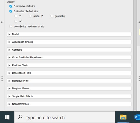
Figure 92: Paired ANOVA: options

To perform the ANOVA analysis for paired samples we have to fill out the following options

Model: automatically filled out -> lists the name of the experimental variable ( = animal -> as filled out in the Repated Measures Factors panel)
Assumptions Checks
- select Sphericity tests
- Sphericity correction -> select None, Greenhouse-Geisser, Huynh-Feldt
Post Hoc Tests -> drag the experimental variable ( = animal) to the right empty panel
- Select Bonferonni
Descriptive plots: drag the experimental variable ( = animal) to Horizontal Axis
- Select display error bars -> confidence interval (95%)

After the settings we will obtain a figure and the p-values for the ANOVA analysis: is there a difference in the mean of the levels?

Go to the Descriptives plot for a visualization of the data
Go to Assumption Checks: Test of Sphericity (Figure 103)

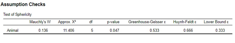
Figure 93: Paired ANOVA: assumptions check output

The p-value of this test is 0,047. This means that the assumption of Sphericity is violated and that the p-value needs to be corrected by the Greenhouse-Geisser or Huynh-Feldt correction factor ( The most extreme correction factor is the lower bound factor, but this will not be used)

Go to the Repeated Measures ANOVA (Figure 104)

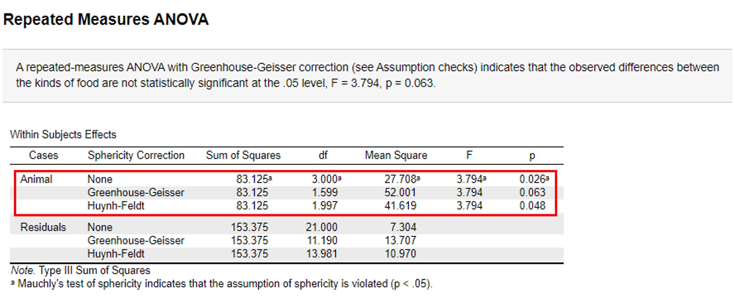
Figure 94: Paired ANOVA: (corrected) p-values

We observe three different p-values (0,026, 0,063 and 0,048). Because the assumption of sphericity is violated we have to use the corrected p-values of 0,063 and 0,048. So now we are left with two p-values leading to the opposite conclusion.

0,063 > 0,05 -> accepts H₀ 0,048 < 0,05 -> accepts H₁

How to deal with this? The p-values are very close to each other. The problem we are facing here is the fact that we use all or nothing thinking about p-values.

P-values depends on the size of your sample (and here the sample is rather small):

With an extreme large sample even very small differences between samples can be statistically significant but biologically completely meaningless
With small samples there could be an true effect (different between sample means) but because of the small sample size we can not show it with a statistical test
Here, there is an indication that there could be a statistical significance difference -> We can therefore repeat the experiment with a bigger sample size.

A more important question is to assess whether the differences that are being observed between the levels of the experiments are biologically meaningful. A small statistical difference between samples could be biologically irrelevant whereas a bigger difference between sample means could be biologically relevant but is not statistically significant.

Therefore never use all or nothing thinking based on p-values and the threshold of 0,05, but evaluate your results in the biological context and compare to what is already know in the literature.

In addition always be transparent in your analysis. Don’t leave out the p-value of 0,063. Include it in your analysis and let the reader decide how to interpret your results. This is part of reproducible science. Imagine, that you would only publish results with a p-value < 0,05. We already know that in the long term we are accepting that 1 out of 20 experiments report false positives. If researcher are not reporting correct p-values or even manipulate p-values the percentage of false reports is even further increased. This is unfortunately common practice and leads to a reproducibility crisis in science.

Go to the Post Hoc analysis:

The pairwise comparisons have been performed with the Bonferonni correction. We observe that there is a difference between “Stick Insect and Kangaroo Testicle” and between “Stick Insect and Fish Eye”.

Althought this is a dummy data set, it is always up to the researcher to interpret this difference in a biological context.

lesson_10_assignment

An oncologist wants to measure the size of colorectal cancer after treatment with a new bio-pharmaceutical. The oncologist selected patients with a stage I tumor with tumor sizes of less then 2 cm. The patients received the new bio-pharmaceutical for a certain time and were measured for tumor size:

sample1: before treatment sample2: after treatment week 16 sample3: after treatment week 32

Copy data file lesson_10_opdracht5.txt from the shared directory to your home directory -> lesson_10
Open the file in JASP
Perform descriptive statistics to test for outliers and normality

Is the data for each group normally distributed?
Does the data contain outliers?
Is the assumption of sphericity violated?
Perform ANOVA analysis and post hoc analysis
What is your conclusion?

Non parametric test

If your sample (n<30) is from a non-normally distributed population the sample mean is not the best estimate to represent the population mean. Because on beforehand we don’t know the population distribution of our variable (= what has been measured), we don’t know how the sampling distribution should look like. Thus, we can not generate accurate confidence interval around the sample mean because these are based on a normal distribution. In this situation we can either use bootstrapping or use non-parametric tests. For each parametric test exists an equivalent non-parametric test (Figure 106).

NOTE: Bootstrapping for parametric tests will not be discussed here, because it uses a different approach in JASP using the linear regression model

In addition, if your level of measurement is not quantitative (ratio or interval, collectively named scale data) but qualitative (nominal or ordinal) we also use non-parametric tests (Figure 105) (these type of data is not common in biological research but more common in social science)

These tests are based on the median values of the data set. The downside is that these tests have less power to observe a true difference between samples (the differences between means should be larger to conclude that it is statistical significant compared to parametric tests)

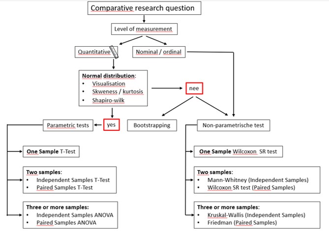
Figure 95: Decision scheme to select a statistical test for comparative analysis

In the T-Test panels the non-parametric test are listed under Tests
In the ANOVA panels the non-parametric test are listed under Nonparametrics

lesson_10_assignment

Open file lesson_10_opdracht4.txt in JASP. We have concluded that the data is not normally distributed. Analyze the data using a non-parametric test

What is your conclusion?

Linear correlation and Regression analysis

So far, we have dealt with comparative research questions and related parametric tests. JASP can also deal with correlation questions and regression analysis (already discussed in the course Statistiek en Excel). Correlation analysis is to check whether an increase of one variable results in the increase / decrease of another variable. For example, is there a correlation between the average daily number of steps and the Body Mass Index (BMI).

Here, we will show how to use JASP to generate correlation plots, calculate the Pearson’s correlation coefficient and the formula of the regression line.

To perform correlation and regression analysis we have to check for the following assumptions:

The level of measurement of both variables are quantitative
Linear Relationship: There should exist a linear relationship between the two variables
Each observation in the dataset should have a pair of values (same number of values for each variable)
Normality of the two variables
No presence of outliers in the data

A researcher wanted to know if there is a correlation between the physical activity (PA) and Body Mass Index (BMI). The data is in file lesson_10_PA_BMI.csv

Copy this files from the shared directory to your home directory -> lesson_10
Open the file in JASP
Inspect the data:

variable1: PA = physical activity -> average daily steps
variable2: BMI

Open a Descriptive panel and check for normality

The samples have n=100. So we don’t have to worry about normality

Within the Descriptive panel -> Basic plots -> Correlation plots

There seems to be a negative linear correlation. Also we don’t observe outliers in the scatter plot which deviates from the trend. Therefore we can perfporm the correlation analysis:

Before we perform Pearson’s correlation test we formulate the hypothesis:

H₀ : There is no correlation between two variables. The correlation coefficient = 0
H₁ : There is a correlation between two variables

Open Regression -> Correlation panel
Fill out the options as shown in Figure 106

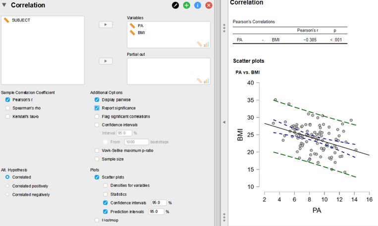
Figure 96: JASP: correlation analysis

The Pearson’s correlation coefficient (r) is -0,385 (showing a negative correlation) with a p-value of < 0,001. If there would be no correlation the r value is 0 and this is the H₀. The p-value associated with the r value is the chance of obtaining the r-value under the assumption that there is no correlation. The bigger the r value the smaller the chance of obtaining this value. In this example we observe a weak to medium correlation but it is still highly significant with a p-value of < 0,001. The reason for this low p-value is that the samples are rather large with n=100. This is a very important point. With large enough samples (correlation and comparative research question) even small correlation / differences which are biologically meaningless can become statistically significant. And the other way, large correlation / differences which could be biologically meaningful2, can become not statistically significant when the samples are small.

Once we have established that there is a correlation we can calculate the regression formula.

The general formula of the regression line: y= Ax + B. To obtain the A and B coefficients:

Go to Regression -> Classical -> Linear Regression
Drag variable PA to the Covariate window
Drag variable BMI to the Dependent Variable
Under the Statistics panel -> Coefficients -> Confidence interval

The formula is listed in the regression output (Figure 107)

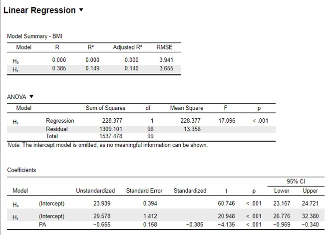
Figure 97: JASP: regression analysis

The first panel shows the Model Summary:
The R² for this analysis is listed under H₁ : 0,149
(Note that the R value in the model summary is the same (positive) value as the correlation coefficient)

The third panel shows the Coefficients:
The A coefficient is listed under Unstandardized (H₁) : -0,655 with a lower limit of -0,969 and an upper limit of -0,340
The B coefficient is the intercept (H₁) : 29,578 with a lower limit of 26,776 and an upper limit of 32,380
(always state the confidence interval for the A and the B coefficients. The confidence interval for the regression line is shown in the correlation output panel -> Scatter Plots -> blue dashed line)

The formula of the regression line with which we can calculate the BMI value (y) based on the average daily steps (x) :
y = -0,655x + 29,578
R² = 0,149

If we make a prediction for the BMI based on the average daily steps we will also have an interval because it is a prediction based on a the regression line of a sample. This is the prediction interval and is shown in correlation output panel -> Scatter Plots -> green dashed line)

There are numerous assays to measure / detect / quantify proteins in cells. Most often this include the use of antibodies which specifically binds to your protein of interest. The antibody can be labelled with a fluorescent tag to visualize and possibly quantify your protein of interest. One such method is “enzyme-linked immunoassay” or in short ELISA.

Using the KEGG pathway map of gastric cancer we have learned that an infection with Helicobacter pylori is a risk factor for gastric cancer. The presence of Helicobacter pylori in the gastric mucosa initiate an inflammation response. Cells of the immune system respond by the excretion of cytokines which are small signalling proteins into the environment. This results in a cascade of further immune activation leading to chronic inflammation and chronic stress on the mucosa.

A researches want to know whether the cytokine TNF\(\alpha\) is secreted in patients with gastric Helicobacter pylori infection.
The researcher collected gastric biopsy samples from patients with Helicobacter pylori infection and a control group of people without infection. The biopsy samples were briefly grown in vitro in the lab and samples were tested for TNF\(\alpha\) secretion using the ELISA assay.

lesson_10_assignment

What is the type of research question?
What is the model system?
What is the outcome variable?

To quantify protein levels , it is required to make a calibration curve. Purified TNF\(\alpha\) is diluted and measured using a spectrophotometer. Using the formula of linear regression, TNF\(\alpha\) concentrations can be calculated for the experimental groups.

The data of the experiment is present in the shared data folder lesson_10. The data consist of two files:

lesson_10_opdracht8_tnfa_calibration.txt
lesson_10_opdracht9_tnfa_patients.txt

Copy these data files from the shared directory to your home directory -> lesson_10
Perform a correlation and regression analysis on the original data

lesson_10_assignment

Are you satisfied wit an R² of 0,950?

The researcher made an error when entering the data.

Restore the error
Save the adjusted file as lesson_10_opdracht8_tnfa_calibration_2.txt
Repeat the correlation and regression analysis

What is the R²?
What is the formula of the regression line?

The extinction of the control group and the patients with Helicobacter pylori infection are in file lesson_10_opdracht9_tnfa_patients.txt

lesson_10_assignment

Calculate the TNF\(\alpha\) levels of the two groups using the formula of the regression line?

In JASP there are two possibilities to calculate the TNF\(\alpha\) levels by creating new columns:

method1:
(1) Add a new column and substract the B value of the formula (y = Ax +B) from the extinction values
-> compute column
(2) Add another column and use the value of the previous column to divide by the A value of the formula -> compute column

method2:
When creating a new column, enter the name of the new column and below the name field, click on the R icon -> Create Column. A new field will pop up with the text (#Enter your R code here :)
On the next line enter:
(extinction - B) / A
-> compute column (The A and the B values are the coefficients of the regression line)

Is there a difference in TNF\(\alpha\) secretion between the two samples? Perform the analysis in JASP.
What is your conclusion?

When two quantitative variables in correlation analysis are not normally distributed we can use bootstrapping or using the Spearman’s rank correlation test.

Spearman’s rank correlation test: correlation panel -> Sample Correlation Coefficient -> Spearman’s Rho (see Figure 106)
Bootstrapping: Linear Regression -> Statistics -> Regression Coefficients -> Estimates -> select the “from 5000 bootstraps”