Lesson_02 - The genome

Learning objectives

The student is able:

• To obtain (genomic) data from http://www.ensembl.org/index.html
  
• To obtain (genomic) data from https://bacteria.ensembl.org/index.html
  
• To analyse (genome) data using the data analysis workflow in JASP
• To organise and transform data using bash

The human genome

To understand human (disease) phenotypes it is essential to understand the human genome. The long lasting molecular quest is to connect a genotype to a phenotype. For example which genes are involved in cell cycle regulation, muscle contraction, immune reaction, development and so on. In a similar way, we want to connect a genotype to a disease phenotype such as cancer or how genotypes of bacteria confer antimicrobial resistance. Mutations in the genome affecting gene function can possibly lead to cellular dysfunction and subsequently adverse health effects. Therefore it was of critical importance to sequence the human genome.

The first version of the human genome was published in 2001 and in 2022 a complete version was published. It was a bit of an disappointment that the human genome contained about 20.000 genes (compared to for example rice which has about 40.000 genes). Within the human genome, distinct functional elements can be defined (Figure 11)

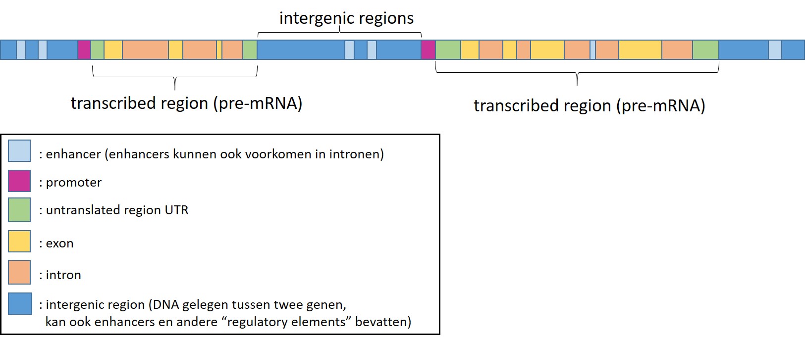
Figure 11: Functional elements of the human genome

Protein coding genes constitutes for about 2% of the human genome. The remaining nucleotides are so called “noncoding DNA”. In recent years it has become clear that parts of these regions are also transcribed in RNA but not translated into proteins (non-coding RNA). Furthermore the human genome contains a lot of “regulatory elements” which control gene transcription (promoters, enhancers, silencers, eRNA) and the 3D structure of the human genome (folding of the genome, which information is / becomes available)

Splicing

The process of splicing (Figure 12) dictates which exons are present in a transcript. Different transcripts from a gene translate into proteins with distinct functions. Thus, although we have about twenty thousand genes they can possibly produce a multitude of transcripts and thus proteins.

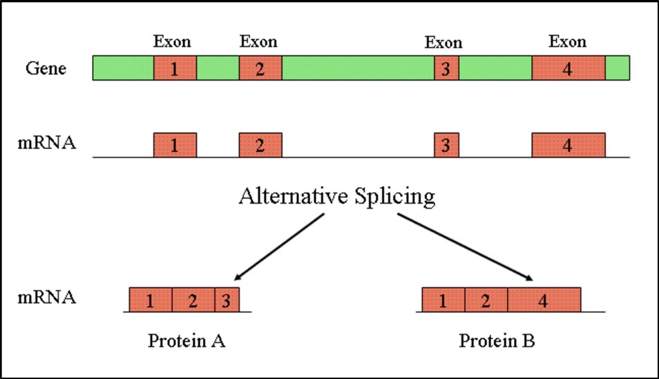
Figure 12: Splicing produces distinct RNA transcripts

Ensembl database

The ensembl database contains information about hundreds of vertebrate genomes including the human genome. With the ensembl BioMart tool we can obtain all genes + associated features of a vertebrate genome.

We will acquire a list of genes of the human genome and start to explore (describe) genome and gene features by using the first 4 steps of the data analysis workflow:

Obtaining data:

• Go to the ensembl database (Figure 13) and select BioMart

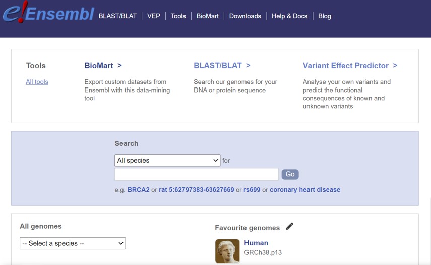
Figure 13: Ensembl database

• Within BioMart (Figure 14)
• CHOOSE DATABASE -> Ensembl Genes 107
• CHOOSE DATASET -> Human genes (GRCh38.p13)

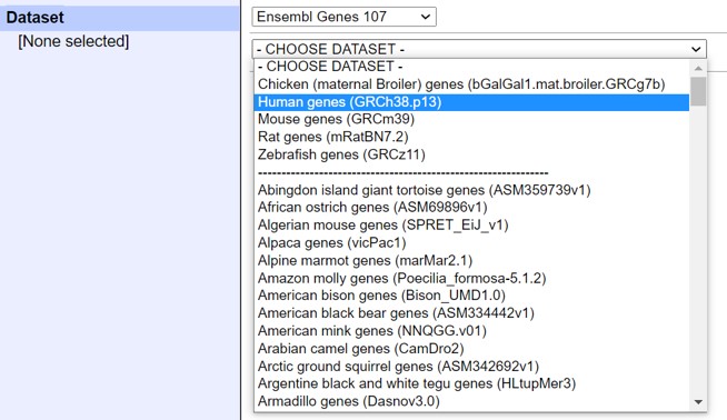
Figure 14: Ensembl dataset selection

• Click on Filters
• Open drop down menu of REGION
• Select 1-22 and X and Y (X and Y are at the end of the list) as shown in Figure 15

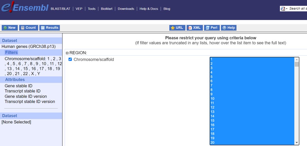
Figure 15: Ensembl Filters selection

• Click on Attributes (left panel)
• Features
• Open drop down menu of GENE
• Select the options as shown in Figure 16

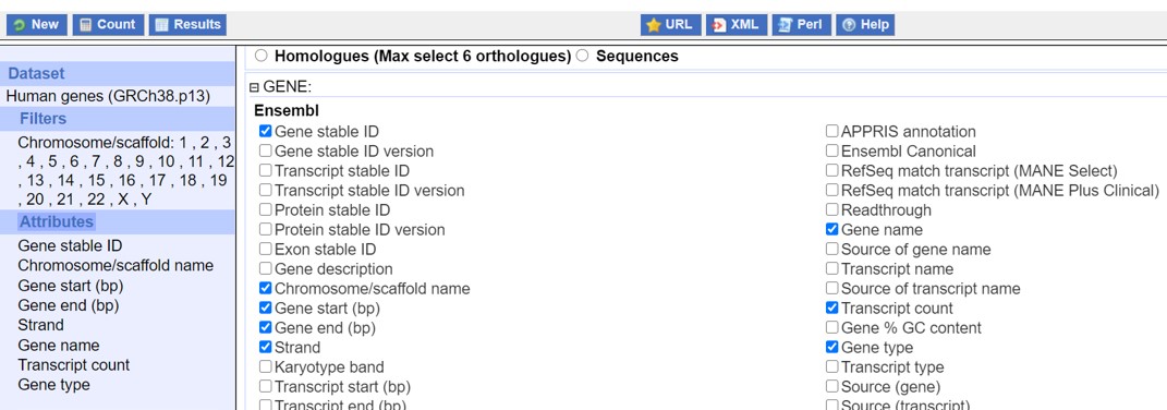
Figure 16: Ensembl Attributes selection

• Click on the left upper panel on Results
• Select as shown in Figure 17 (Don’t forget to check “Unique results only”)
• Click on GO
• The data file will be downloaded to your computer

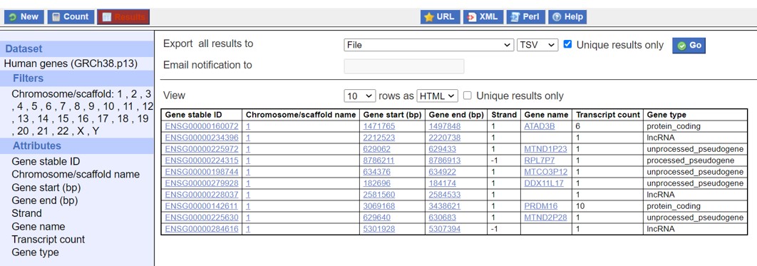
Figure 17: Ensembl data output download

• Rename the data file mart_export.txt to lesson_02_opdracht1-2_ensembl_GRCh38.txt
• upload the ensemble file to your home directory-> lesson_2

JASP

Excel is commonly used for data analysis. Excel is useful for early steps in data cleaning and organisation. Excel is also very useful as a calculator. However (big) data analysis in Excel is often very laborious and more importantly data analysis in Excel is not reproducible:

• Reorganizing data in Excel increases the chance of making mistakes
• No warnings are issued when you make a mistake, for example when copied formulas are applied to the wrong columns
• No debugging options in Excel
• Excel tends to auto format text so original descriptions get lost (for example numbers could be changed to a date!!)
• Excel is limited to about one million rows. Not suitable for big biological data sets
• Speed of computation for complex data transformations is very low and could cause computer crashes
• The steps you take in Excel are not documented. Therefore it is not clear how you reached a certain conclusion
• Lack of automation: if you have to repeat the analysis in a slightly different way on the same data or in a similar way on a different data set you have to start all over again because the steps were not documented
• Difficulty in collaboration. Simultaneous working on data analysis, commenting and sharing of data files is not possible in Excel. Different versions of Excel on windows / Mac can already give problems in data transfer

For reproducible data analysis we have to use alternative software to document all the data analysis steps which have been used to generate graphs, statistical tests and conclusions. It is important that these software alternatives are free of charge so everyone can download and repeat your analysis using the same software. Here we will make use of JASP. We will also use bash and R. JASP can be installed on your computer from the HU software center or otherwise from the JASP download page.

Data import

JASP is an open source statistical program based on the R language. Using JASP we can easily perform descriptive statistics, parametric and non-parametric tests as well as correlation and regression analysis. JASP accepts different types of data files:

1. JASP files
2. txt files

• csv files (comma separated values)
• tsv files (tab separated values)

3. ods files (open document spreadsheet)

Ods files are from libreoffice. Libreoffice is a free alternative to microsoft office to promote open science. Within Excel you can save data files into the ods file format.

To demonstrate JASP we will continue with the ensembl human gene data file lesson_02_opdracht1-2_ensembl_GRCh38.txt.

• Open JASP
• Click on the 3 three blue lines (upper left) -> Open -> Computer -> Browse
• Browse to the folder containing the ensembl data file

Data inspection

After importing the data file it should look like Figure 18

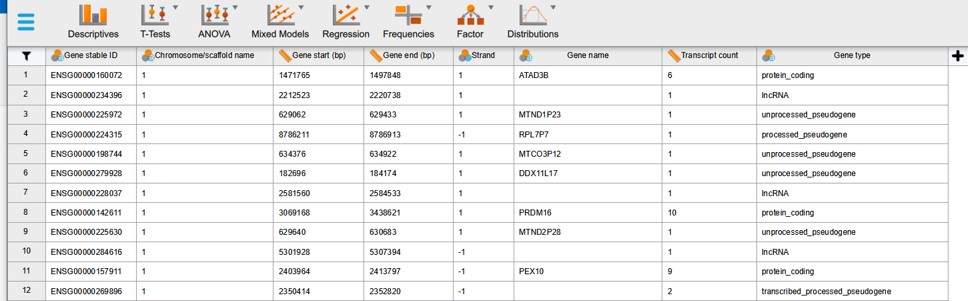
Figure 18: Ensembl data in JASP

Data filtering

Each column name starts with a pictogram indicating the type of data (nominal, ordinal or quantitative). To check which categories are present in a column with nominal data click for example on the column name “Gene type”. On top of the data a list will appear with the unique values of that column. We observe (after simple counting) that there are 38 different gene types (Figure 19).

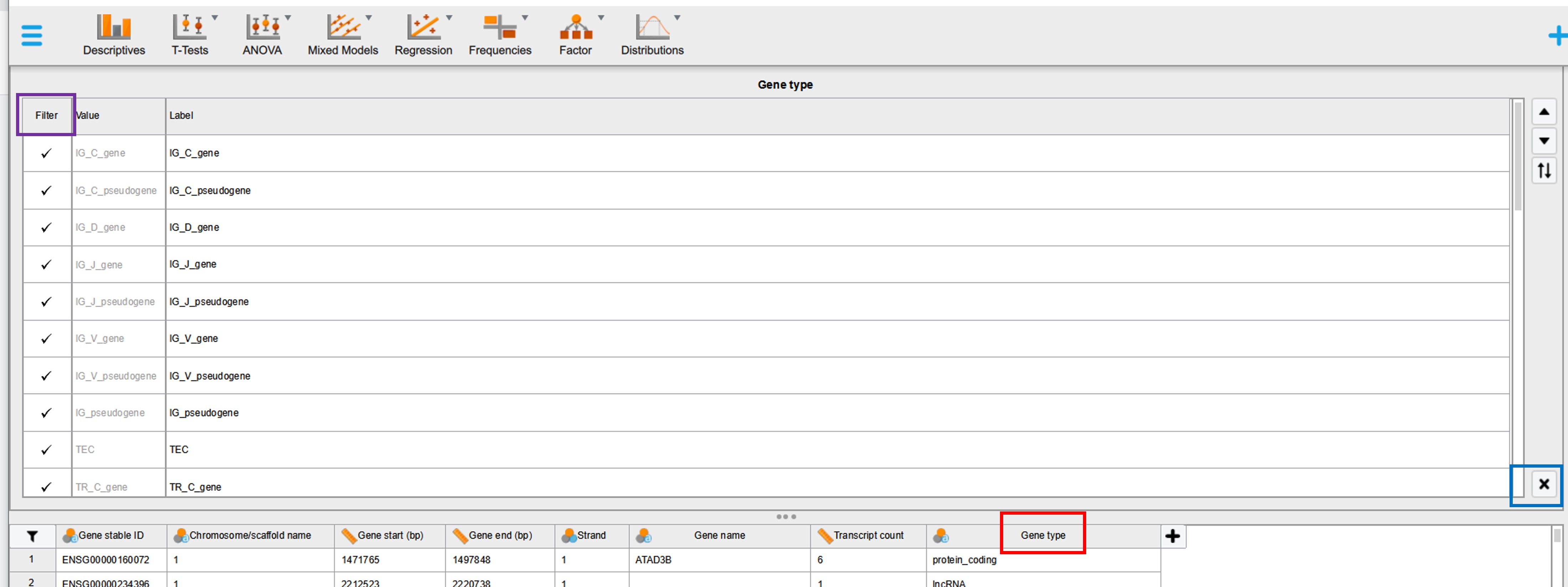
Figure 19: JASP filtering options

On the left hand side it is possible to select (filter) categories of interest by un-checking categories that should not be part of the analysis (Figure 19, purple rectangle). For example we can compare the properties of protein_coding, lncRNA and miRNA gene types (in stead of all 38 different gene types). Click either on the black cross (Figure 19, black rectangle) or again on the column name (Figure 19, red rectangle) and the window will disappear.

Descriptive statistics

We can now easily calculate all kinds of descriptive statistics for this data file. Before we start the analysis we have to think about interesting research questions and our experimental setup. Our research model is the human genome. We have observed that there are 38 different gene types in the human genome. We can consider these categories as our experimental groups or experimental variable. For each group we want to know their properties (=outcome variable), for example the average number of transcripts:

“Gene type” (= experimental variable) -> human genome (model) -> “Transcript count” (= outcome variable)

• Click within the top menu on the “Descriptives” button
• Select “Gene type” (= experimental variable) and drag to the “Split” window (Figure 20)
• Select “Transcript count” (= outcome variable) and drag to the “Variables” window
• Click on “Transpose descriptive table” (for easier view of the table)

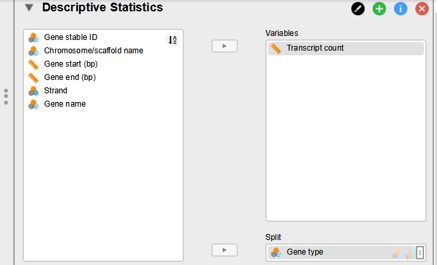
Figure 20: JASP variable selection

To add the median to the descriptive table:

• Click on the “Statistics” (left panel lower part)
• Select the median option (Figure 21)

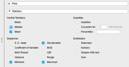
Figure 21: Statistics option panel

In the “Results” panel we see a descriptive summary of “Transcript count” for each type of gene. The line “valid” counts how many cases are in each category of “Gene type” (Figure 22)

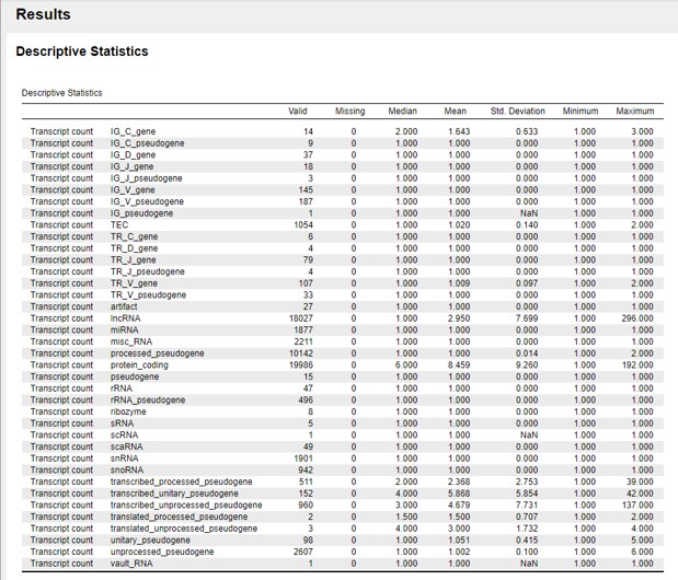
Figure 22: Descriptive statistics output

lesson_02_assignment

Clean up the results section to only show the following “Gene type” categories:

1. protein_coding
   
2. lncRNA
   
3. miRNA

1. How many protein_coding, lncRNA and miRNA genes are present in the human genome?
2. What is the median transcript count of protein_coding, lncRNA and miRNA genes?
   
3. What is your conclusion of (B)
   
4. In JASP, save the file as lesson_02_opdracht1-2_ensembl_GRCh38.jasp

Creating new variables

Within JASP we can calculate a new variable based on existing variables. Here, we calculate the gene length which is the difference between the variables “Gene end (bp)” and “Gene start (bp)”.

• To add an extra column (= variable) click on the + sign next to the last column (Figure 23)

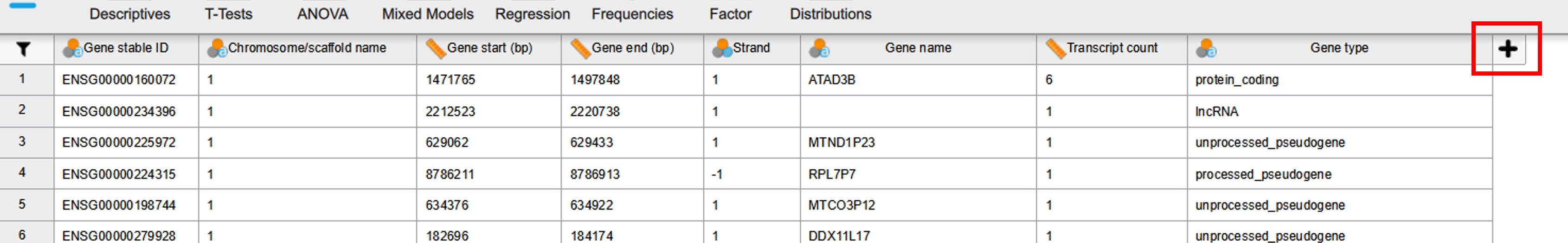
Figure 23: Add new column in JASP

• Fill in the name of the column. In this case “Gene length” (Figure 24)
• Click on “Create Column”

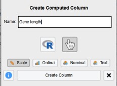
Figure 24: Add new column name

• Calculate the formula by dragging the variables “Gene end (bp)” and “Gene start (bp)” in the formula box. Don’t forget to put the minus sign in between (Figure 25)
• Click on “Compute Column”

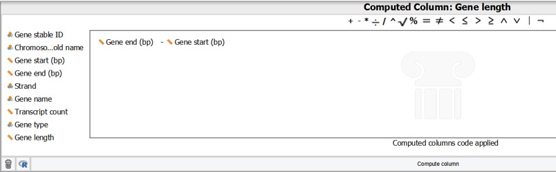
Figure 25: Formula box to create a new column

• Click on the black cross (lower right of the formula box) to close the formula window

---

NOTE : Within a data file you can perform many different descriptive analysis. For each Descriptive analysis you can open a new “Descriptive Statistics” panel (Figure 26). To rename each tab click on the black circle icon with pen. Write a new informative name and press enter.

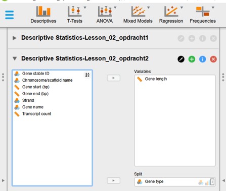
Figure 26: Multiple descriptive analysis tabs in JASP

lesson_02_assignment

• Click on “Descriptives” to open a new “Descriptives” tab
  
• Rename the tabs of assignment 1 and 2 as shown in figure 26

1. Calculate the average (mean) “Gene length” of protein_coding, lncRNA and miRNA genes?
   
2. What is your conclusion?
3. Save the file in JASP and upload the file to your home folder -> lesson_2

There are more gene characteristics we can study. In Biomart it is possible to select a range of options

• Go to the ensembl biomart database as before and add the following attributes to the human genome:

1. Transcript length (including UTRs and CDS)
2. Gene % GC content

• Check if you have still selected chr1-22 and X and Y
• Check if you have selected 10 attributes in total (8 of the previous analysis + 2 extra)
• Download the data
• Rename the data file mart_export -> lesson_02_opdracht3-4_ensembl_GRCh38.txt
• Open the data in JASP
• Filter the data file for protein_coding, lncRNA and miRNA type genes

lesson_02_assignment

A researcher wants to calculate the average (mean) transcript length for each of the three Gene types (we already have calculated the average gene length, see assignment 2)

“Gene type” (= experimental variable) -> human genome (model) -> “Transcript length (including UTRs and CDS)” (= outcome variable)

• Open a new descriptive tab
  
• Name the tab “Descriptive Statistics-Lesson_02-opdracht3”

1. What is the average (mean) “Transcript length (including UTRs and CDS)” of each gene type?
2. Compare the values of (A) to the average “Gene length” (see assignment 2)
3. What is your conclusion?
   
4. In JASP, save the file as lesson_02_opdracht3-4_ensembl_GRCh38.jasp

Another important feature of the genome is the % GC content. For example species have different % GC content in their genomes. Also within a genome there are marked differences of GC content between the different genome elements such as genes, non_coding DNA, teleomeres and centromeres.

lesson_02_assignment

A genome researcher wants to know the average (mean) “Gene % GC content” for each chromosome:

“Chromosome/scaffold name” (= experimental variable) -> human genome (model) -> “Gene % GC content” (= outcome variable)

• Open a new descriptive tab
  
• Name the tab “Descriptive Statistics-Lesson_02-opdracht4a”

1. Which chromosome contains the highest mean “Gene % GC content”?

A genome researcher wants to know whether “Gene % GC content” is normally distributed for protein_coding, lncRNA and miRNA genes:

“Gene type” (= experimental variable) -> human genome (model) -> “Gene % GC content” (= outcome variable)

• Open a new descriptive tab
  
• Name the tab “Descriptive Statistics-Lesson_02-opdracht4b”

2. Are the “Gene % GC content” for each type of protein_coding, lncRNA and miRNA gene normally distributed?

HINT: Open the “Plots” menu within Descriptive Statistics and select the correct figure type

3. Save file in JASP and upload the file to your home folder -> lesson_2

The bacterial genome

The bacteria.ensembl database contains information about thousands of bacteria and archaeal genomes. A bacterial genome is very differently organised compared to eukaryotic genomes.

Features of a bacterial genome:

1. single circular DNA molecule (in cytosol)
2. includes plasmids
3. haploid

A researcher want to know how the genome of bacteria and vertebrate are structured and if there are marked differences. First, let’s calculate the gene density of the Helicobacter pylori genome and the human genome. The Helicobacter pylori is becoming increasingly resistant to antibiotics and causes a variety of (serious) health problems. The gene density is defined by the number of protein coding genes per million bp. Thus, we need to obtain two characteristics of the genomes.

1. Total length of the genome
2. The number of protein coding genes

Go to the bacterial ensembl database (Figure 27)

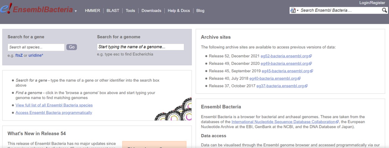
Figure 27: Bacterial ensembl database

• In the “Search for a genome” box type Helicobacter pylori
• Click on any Helicobacter pylori with TaxID 210 (It doesn’t matter which one, the genome length and number of protein coding genes are more or less in the same range)
  
• Click on “More information and statistics” (Figure 28)

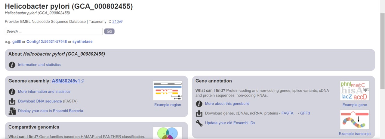
Figure 28: Bacterial ensembl genome summary

• Retrieve the number of protein coding genes and genome length (Golden Path Length)
  
• Obtain genome length and number of protein coding genes of the human genome (as describes for the bacterial genomes but use the vertebrate ensembl database.

lesson_02_assignment

Calculate the gene density in the Helicobacter pylori genome and the human genome?
What is your conclusion?

We observe that there is a difference in gene density between prokaryotic and eukaryotic genomes. As a researcher we want to know why? Can we explain this difference by the way these genomes are organised? Let’s further inspect the Helicobacter pylori genome using the bacterial ensembl database (see previous assignment):

• Click on GFF3 link (Figure 28)
• Click on the Helicobacter pylori link

You have downloaded data file Helicobacter_pylori_gca_000802455.ASM80245v1.49.gff3.gz. The General Feature Format (GFF) is a tab-delimited text file that holds information on genes. Notice that the files end on .gz meaning that the file is zipped.

• Transfer the file to directory lesson_2 within your home directory

Data analysis using bash

Bash contains numerous commands that can be used for data inspection, cleaning, organization and analysis. The advantages using bash are:

• With (a few) bash commands we can inspect, clean, organize and analyse data files
• Bash commands can be saved in a script for reuse and reproduction
• Data analysis workflow can be automated for multiple input files

Bash: tab-completion

The name of our data file is Helicobacter_pylori_gca_000802455.ASM80245v1.49.gff3.gz. This is a very long and complicated name. It will take a lot of time to type this file name in the terminal and probably we will make a mistake. But bash has an elegant solution for this problem (bash has a solution for everything!)

Bash has a useful feature namely tab-completion. If you press TAB after you have written the first 1 or 2 letters of a folder, file or function, Linux automatically fills out the name. If the name is not unique, Linux will show all names that start with the entered letters. For example, if you enter “le” and then press TAB, you get “lesson”. If you then press TAB again you will see all names that start with lesson:”lesson_1, lesson_2, lesson_3 and so on. This way you will see all folders that start with “lesson”. Add _1 to “lesson” (lesson_1) and press enter. This way you don’t have to write out the whole name in the terminal but only a few letters supplemented with the TAB function. It is important that you understand this and can apply it. In the remainder of this course we will work with long file names and it is inconvenient to type them in completely each time. It is also error prone. The Tab Complement automatically searches for the correct files.

NOTE: If tab-completion doesn’t work, it means that either the file doesn’t exist or you’re working in the wrong directory!

Data inspection using bash

Before we can clean and organize the data we have to know how the data is organized. The first step of the data analysis workflow is data inspection.

Bash: gzip

• Go to directory lesson_2 (with the cd command)

Most genomic data are zipped to save space. A zipped file has a .gz extension. Before we can inspect and clean the data file we have to unzip the file. To unzip a data file we use the gzip command:

• To unzip a file we use gzip in combination with the -d option ( = decompress)

gzip -d Helicobacter_pylori_gca_000802455.ASM80245v1.49.gff3.gz

NOTE: use tab-completion to fill out the file name of Helicobacter_pylori_gca_000802455.ASM80245v1.49.gff3.gz. Just enter the first 2-3 letters of the file name and press tab. The rest of the file name will be filled out automatically. Be sure to be in the right folder.

NOTET: if we want to zip a file we use gzip in combination with the -9 option ( = compress better)

gzip -9 Helicobacter_pylori_gca_000802455.ASM80245v1.49.gff3

Bash: rename a file with mv

To rename a file using the bash terminal we will use the mv command. The mv command is used to move a file to another directory. But it can also be used to rename a file by adding a new file name

mv old_filename new_filename

We will rename file Helicobacter_pylori_gca_000802455.ASM80245v1.49.gff3.gz into lesson_02_opdracht5_Hpylori.gff3

mv Helicobacter_pylori_gca_000802455.ASM80245v1.49.gff3 lesson_02_opdracht5_Hpylori.gff3

Bash: word count

How do we inspect a data file on the server? There are a couple of bash commands which are very handy for data inspection

To count the number of lines of a file we use the wc command (word count). The wc command counts the number of characters, words and lines of a file. To count the number of lines we use the -l (lines) option:

wc -l lesson_02_opdracht5_Hpylori.gff3

lesson_02_assignment

How many lines are present in data file lesson_02_opdracht5_Hpylori.gff3

Bash: head and tail

The head command shows by default the first 10 lines of a file:

head lesson_02_opdracht5_Hpylori.gff3

If we want to change the number of lines shown we can add the -n option followed by a number. To show the first 50 lines of a data file:

head -n50 lesson_02_opdracht5_Hpylori.gff3

---

The tail command shows by default the last 10 lines of a file. Similar as with the head command we can use the -n option to change the default setting. To show the last 100 lines of a file:

tail -n100 head lesson_02_opdracht5_Hpylori.gff3

bash: combining commands in a pipeline (part 1)

It is also possible to combine bash commands.

The output of the first command serves as input for the second command

data -> command1 -> output1 -> command2 -> output2

The sequential use of bash commands is called a bash pipe or pipeline and is very common in bash programming. To make a bash pipeline we use the pipe symbol also known as the vertical line (|)

Generally to make a bash pipeline use the following syntax

command1 -options file | command2 -options

---

To exactly show line 76 of data file lesson_02_opdracht5_Hpylori.gff3 we can first select the first 76 lines with the head command and use that as an input for the tail command to only show the last line.

head -n76 lesson_02_opdracht5_Hpylori.gff3 | tail -n1

lesson_02_assignment

What is the bash code to show line 76 and 79 of the data file lesson_02_opdracht5_Hpylori.gff3

lesson_02_assignment

Line 76 to 79 shows the start end end coordinates of the mRNA, exon and CDS of a bacterial gene. Why is there no difference in length between “gene”, “mRNA”, “exon” and “CDS“?

Bash: less

If we want to scroll through a file we can use the lesscommand. The -N option numbers the lines while scrolling

less -N lesson_02_opdracht5_Hpylori.gff3

• If you press enter the file will move one line
  
• If you press the space bar or page up/down all lines shown in the window will move
  
• To leave the less command press q

lesson_02_assignment

Use the less command to scroll down the Helicobacter_pylori data file. The first 67 lines start with a pound sign (# sign) and consist of four columns with genome information. The first line with gene information is line 68. Scroll to line 68

1. How many columns are in line 68?
   
2. Which columns contain the start and the end position of the gene?

Data organisation and transformation using bash

After data file inspection we should have a good idea about how the data is organized and how we can clean the data file. How we organize our data file depends on the research question. What do we want to calculate. In assignment_6 we concluded that bacterial genes don’t have introns. Thus genes are much smaller in bacteria compared to eukaryotic genomes. An interesting question is to calculate whether gene transcripts differ in length between pro- and eukaryotic genomes?

“eu- or prokaryote” (= experimental variable) -> genome (model) -> “Transcript length (= outcome variable)

If we want to calculate the average transcript length (mRNA) we only want lines and columns with mRNA information (for example line 69). To select specific lines and columns in a data file we can use the bash grep and the cut commands

Bash: grep

The grep function searches for patterns in each line of a data file and print out the lines containing the pattern on the screen. The grep commands has many options and can search for very complicated patterns. More on that later in the course

Generally, the grep command works as follows:

grep "pattern" file

It is also possible to select lines not containing the pattern with the -v option (select non-matching lines)

grep -v "pattern" file

---

To select lines containing mRNA:

grep -i "mRNA" lesson_02_opdracht5_Hpylori.gff3

We have added the -i option. Because on forehand we don’t know whether the word mRNA is written as mrna, mRNA, MRNA or perhaps MrNa. Because bash is case sensitive and we want to capture all lines containing the word “mRNA” we use the -i option which make the search case insensitive. In other words, it matches all variants of the pattern “mRNA” with or without capital letters

The output is printed to the screen. That is not very useful. If we want the output in a new file we have to re-direct the output to a new file. We can do that with the > sign followed by the name of the new file

grep -i "mRNA" lesson_02_opdracht5_Hpylori.gff3 > lesson_02_opdracht10_Hpylori_filtered_1.gff3

A new file has been created in your working directory (should be lesson_2). NOTE: The file name has changed from opdracht5 to opdracht10 in the file name!

• Use the head command to check whether each line contain mRNA.

Next we use the data file lesson_02_opdracht10_Hpylori_filtered_1.gff3 to get rid of columns that will not be used in the JASP analysis

Bash: cut

To select columns of a data file use the cut command with the -f option ( = field option). The most relevant columns for our data analysis are the first 5 columns. To select the first five columns of our data file:

cut -f1,2,3,4,5 lesson_02_opdracht10_Hpylori_filtered_1.gff3 > lesson_02_opdracht10_Hpylori_filtered_2.gff3

• Use the head command to check whether there are only 5 columns left in your data file lesson_02_opdracht10_Hpylori_filtered_2.gff3 (Figure 29)

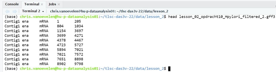
Figure 29: Cleaned GFF3 file

bash: combining commands in a pipeline (part 2)

We have cleaned the GFF3 data file with the bash grep and the cut commands. In the process of data cleaning we produced an intermediate file Hpylori_filtered_1. To remove this file use the bash rm command

rm lesson_02_opdracht10_Hpylori_filtered_1.gff3

To avoid creating extra files (which we don’t use any further) we can combine the grep and the cut commands in a bash pipeline:

grep -i "mRNA" lesson_02_opdracht5_Hpylori.gff3 | cut -f1,2,3,4,5 > lesson_02_opdracht10_Hpylori_filtered.gff3.txt

NOTE: we added txt to the file name. Otherwise it will not be recognized by JASP in the next assignment!

• Also remove file lesson_02_opdracht10_Hpylori_filtered_2.gff3
• Continue with file lesson_02_opdracht10_Hpylori_filtered.gff3.txt

There is one more thing we have to fix. We have to add columns names to the output file. JASP by default expects column names. To add column names to the file lesson_02_opdracht10_Hpylori_filtered.gff3.txt run the following bash command (you don’t have to understand this codes for now)

sed -i '1s/^/contig\tsource\ttype\tstart\tend\n/' lesson_02_opdracht10_Hpylori_filtered.gff3.txt

• Export file lesson_02_opdracht10_Hpylori_filtered.gff3.txt to your computer
  
• Import the data file in JASP

lesson_02_assignment

1. Calculate the average transcript (mRNA) length of genes in the Helicobacter pylori genome
   
2. Compare your result to the average transcript length of human genes (see assignment 3?
   
3. What is your conclusion?
4. In JASP, save the file as lesson_02_opdracht10_Hpylori_filtered.gff3.jasp
5. Upload the file to your home folder -> lesson_2

Thus, based on the answers of the two above questions we have discovered that the bacterial genome of Helicobacter pylori is differently organised. There is actually a third reason. There are hardly any large regions of non-coding DNA between genes; genes are placed very close together in the bacterial genome.

Bash: script

We have observed that the genome of Helicobacter pylori is differently organized compared to the human genome. But this is only one bacterial genome. The genome of Helicobacter pylori could perhaps not be representative of other bacterial genomes. Here, we provide a bash script to automate the data file cleaning + calculation of the average mRNA length of multiple input files.

In bash, if you want to repeat the same analysis you’ll have to type the bash commands again. To avoid retyping bash command, we write a bash script. A bash script is a file which contains all the different steps you want to execute. The name of a bash script always end with .sh. This way we only have to run the bash script and the terminal will execute all the different bash commands:

---

IMPORTANT: To record all the steps of your analysis in a script is the essence of reproducible science. Everyone can see which data analysis steps you performed on your data and by sharing your script and the original input data file, other people can reproduce your data analysis!

---

Generally, to execute a bash script:

bash name_of_bash_script.sh

To store the output of a script in a new file:

bash name_of_bash_script.sh > name_of_file

lesson_02_assignment

In the shared directory lesson_2 are two bash scripts

• Copy these scripts to your home directory
• Run these scripts in the terminal

What is the output of the scripts?

In the shared folder, directory lesson_2 is a sub-directory called assignment_12

• Go to the shared directory and inspect the contents of directory assignment_12
  
• Copy all files from the shared directory to your home directory (to copy a directory + contents use the -r option)

The script3.sh file contains instructions to

• automatically read a GFF3 file (data import)
  
• clean the GFF3 file (data cleaning and organisation)
  
• calculate the average mRNA length (descriptive statistics)

The complete code can be seen in Figure 30.

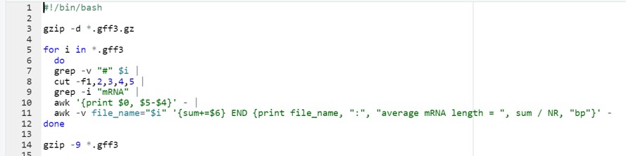
Figure 30: Bash script

lesson_02_assignment

• Run script3.sh in the terminal

What is your conclusion?