Lesson_06 - Gene expression analysis

Learning objectives

The student is able:

To explain the principle of a real time PCR reaction
To design primers for qRT-PCR by using online primer design tools
To analyse qRT-PCR data using the \(\Delta\Delta\)Ct method
To organize and transform RNA-seq data in JASP

Gene expression

Each cell in our body contains the same set of genes. However, there more then 300 different types of cell types (Figure 57). How can we obtain from a single genotype (our genome) more then three hundred different phenotypes (cell types).

Figure 57: Different cell types

The answer is that not all genetic information is transcribed in a cell. Each cell transcribes a number of genes that are required to perform basic cellular tasks to maintain cell viability, the so called house keeping genes. Those genes are not specific for a certain cell type but are expressed in all cells. Besides the house keeping genes, a cell also expresses a specific set of genes in a spatiotemporal manner that determine the function of the cell, the so called cell type specific genes. For example the gene troponin T TNT is specifically expressed in heart cells and the ITGAM gene is specifically expressed in myeloid cells such as macrophages. Some genes are expressed in a very short time window during development. Each cell type expresses a unique combination of genes that determines its function. Theoretically, if we assume a gene is in an on or off state the number of possible gene combinations in a cell is 2²⁰⁰⁰⁰ (20000 is the number of genes).

Stem cells have the potential to give raise to specialized cell types. For example, blood stem cells divide asymmetrically, with one cell retaining the properties of stem cells and the other cell having the properties of a newly differentiated blast cell that continues to divide. The blast cells then differentiate into specialized cells (Figure 58).

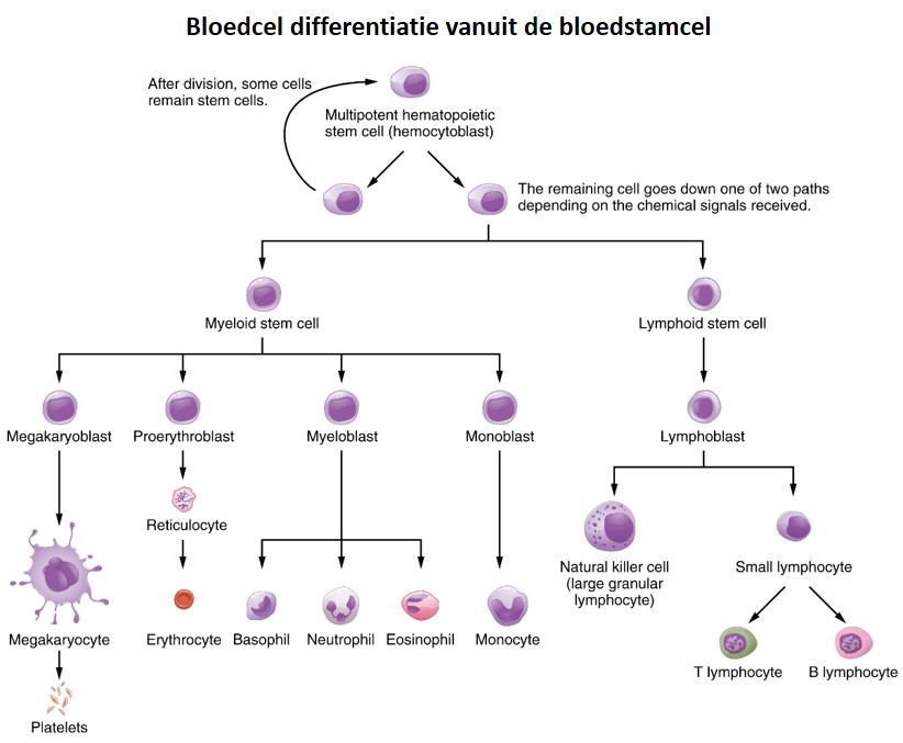
Figure 58: Blood cell differentiation

A gene that plays a role in lymphoid differentition is Pax5. The Pax5 protein acts as a transcription factor and binds the enhancers and promoters of lymphoid specific genes inducing gene expression. If the Pax5 gene is not correctly expressed or the Pax5 protein doesn’t function properly the precursor lymphoid cells fail to differentiate into functional blood cells and they keep on proliferating in an uncontrollable manner leading to Acute Lymphoblastic Leukemia (ALL). Thus, cells with different phenotypes have different gene expression profiles. To understand the relation between genotype and phenotype we have to measure:

Which genes are transcribed in a cell type?
What is the level of mRNA of transcribed genes?

There are two common techniques to measure gene expression:

quantitatively real time PCR (qRT-PCR) to measure the transcripts of a selection of genes
RNA-seq to measure all transcripts in a cell

qRT-PCR general principle

First all mRNA is isolated from cells and converted to cDNA (Figure 59). To single out our transcript of interest from the pool of all transcripts, specific primers are designed to amplify the transcript in a PCR reaction. This is an important step. You have to make a decision which genes you want to analyze. Because on beforehand you make a gene selection, this approach is biased.

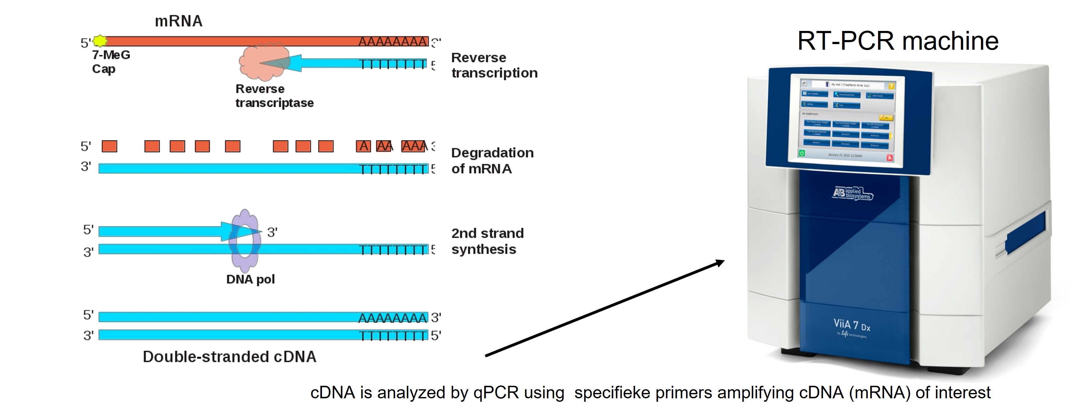
Figure 59: Conversion of mRNA to cDNA

Primers, polymerase, cDNA and a fluorescent chemical (sybr-green) are mixed together and placed in the PCR machine. In each cycle of the PCR reaction the forward and reverse primer hybridize with the target cDNA and polymerase copies the DNA strand thereby doubling the amount of targeted DNA. The other DNA is not amplified (at least if your primers are very specific and only bind to the target DNA). Sybr green only binds to double strand DNA and after each cycle the fluorescent signal is measured by the PCR machine. Because after each cycle the targeted DNA is doubled, there will be an exponential amplification of the targeted cDNA until the amount of primers, sybr-green and polymerase activity decreases and the signal gets saturated (Figure 60).

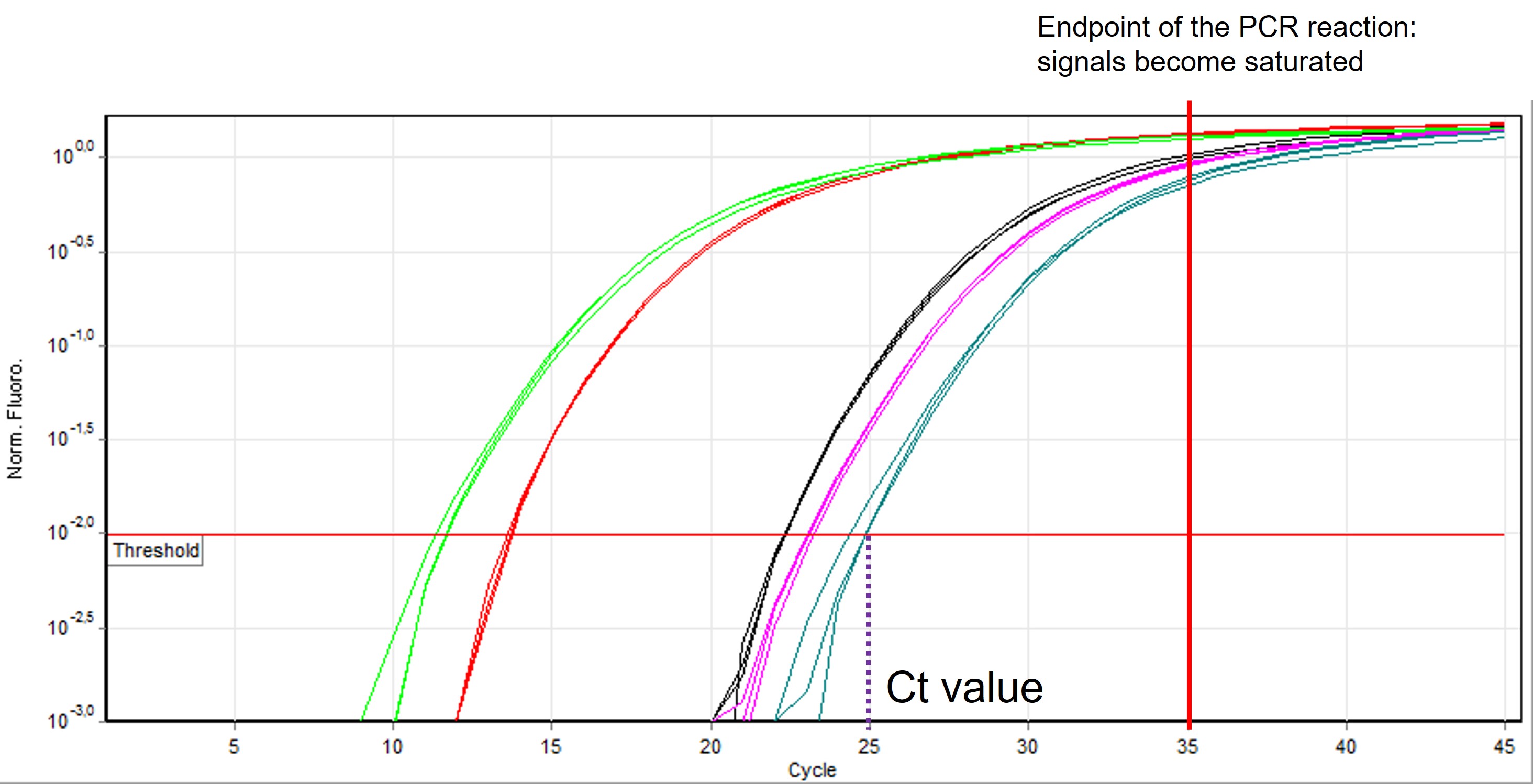
Figure 60: qRT-PCR output curve

After the qRT-PCR reaction has finished, the software draws a threshold line (or you can do it manually) across the samples in the (early) exponential phase of amplification (Figure 60, red horizontal line). The threshold line indicates a level of fluorescence above background levels. Based on this line a Ct value is calculated for each sample which represent the number of cycles to reach the threshold value ( see Figure 60, vertical dashed purple line). In other words, this value tells how many cycles it took to detect a real signal above background levels from your samples.

IMPORTANT: A lower Ct value means that there is more abundance of your targeted DNA. If you start with more cDNA fragments of your transcript of interest in your sample it takes less cycles to reach the threshold. Ct values are on a logarithmic scale. A difference of one Ct value (for example, sample 1 has a Ct value of 25 and sample 2 has a Ct value of 26) means a difference of one Ct value which is 2¹ = 2 times the amount of cDNA between samples (and a difference in Ct values of two = 2² = 4 times more the amount of transcript)

NOTE: Using the classic method of PCR, nucleotides are amplified and visualized on an agarose gel. This means that we only measure the end-point of the reaction where the signal gets saturated and differences are not longer measurable (See Figure 60, red vertical line). Therefore, this method is not suitable to quantitatively measure expression levels.

qRT-PCR control

To interpret the gene expression results using qRT-PCR we have to include the right controls. This is an important step in experimental design to include control samples. Without your controls you can’t interpret your results!

Negative control: Include a sample that contain water instead of cDNA. We don’t expect to detect any signal here because there is no cDNA to amplify. However, if we do see a signal we can conclude that our reagents to set up a PCR reaction are contaminated with nucleotides
Positive control: Include a previous cDNA sample and primers of which you know that they work in a qRT-PCR (from previous experiments). If you don’t detect any signal you can conclude that you made a mistake in setting up the reaction or that one of the reagents is not working properly (perhaps your co-worker left the polymerase too long on his bench and there is no enzymatic activity left)
Loading control: Include a set of primers which target a gene that will not change in gene expression levels between all samples

To further explain the importance of a loading control let’s consider the following experiment. A researcher wants to test whether the addition of a drugs activate a certain gene. The researcher has two groups:
1. control group: no drugs added 2. treated group: drugs added

The gene that is measured is here generally calles “transcript”. The data is present in Figure 61 and doesn’t include a laoding control

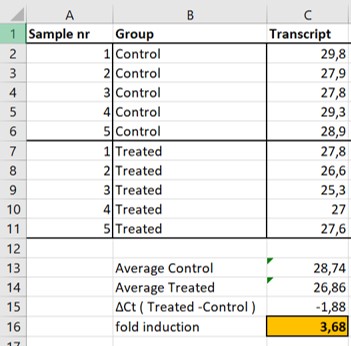
Figure 61: non-normalized expression levels of two transcripts

To analyse the data we calculate:

The average Ct values of the Control samples (Cell C13) and the Treated samples (Cell C14)
The difference ( difference = greek symbol \(\Delta\) ) between the Treated group and the Control group (Cell C15)
The fold induction with the following formula 2^{-\(\Delta\)(Treated-Control)} (Cell C16)

We observe that on average it took samples of the Treated group 1,88 less cycles (Cell C15) to reach the threshold compared to the Control group. Because each cycle represents a 2 fold difference in the amount of transcripts we can make the following calculation: 2^-(-1,88) = 3,68. Thus, we conclude that there is on average 3,68 times more transcript in the Treated samples compared to the Control samples

IMPORTANT: Don’t forget the minus sign because there is an inverse correlation between Ct values and the amount of transcript in your sample. The lower the Threshold value the more transcripts are present in your sample!

But is this correct! There is an alternative explanation. If we start out with more cDNA in our PCR reaction we will also obtain lower Ct values. This difference is therefore not biological relevant but simply a consequence that there was more cDNA to start with. Perhaps you made cDNA of the Treated samples on day 1 and the Control samples on day 2 (not a good idea. You want to keep all technical conditions the same. Therefore it is best practice to prepare all your sample at the same time with the same reagents and equipment). Perhaps you made a wrong dilution for the Treated samples.

Therefore we have to normalize our data. In order to do so, in parallel a house keeping gene (HKG) is measured for each sample (figure 62, column HKG). House keeping genes are stably expressed at high levels and are presumed not to change within samples and conditions. If we observe different Ct values of the house keeping gene between the Control and the Treated samples we can conclude that we started out with different concentrations of cDNA in our experiment. To analyse our data including the loading control values we use the \(\Delta\Delta\)Ct method.

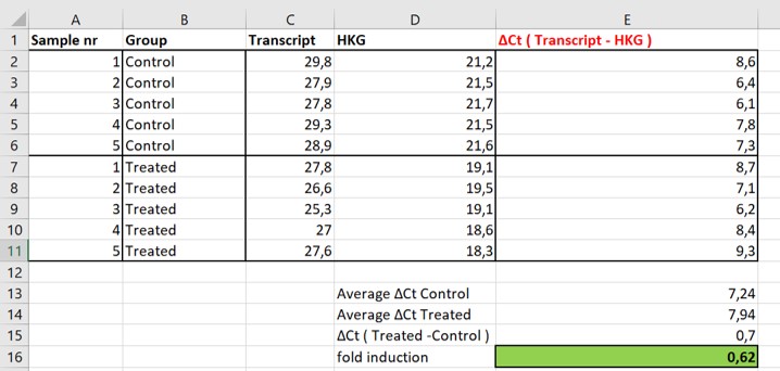
Figure 62: normalized expression levels of two transcripts

\(\Delta\Delta\)Ct method

Before we calculate the average difference in Ct values between the Treated and the Control group we first normalize the Ct values based on the HKG values (Figure 62)

Calculate for each sample the difference between the Ct values of the Control / Treated samples and the HKG Ct value (C2:C11-D2:D11 = E2:E11)
Calculate the average normalized Ct values of the Control (Cell E13) and the Treated (Cell E14) group
Calculate the difference between the Treated group and the Control group (Cell E15)
Calculate the fold induction with the following formula 2^{-\(\Delta\)(Treated-Control)} (Cell E16)

We observe that on average it took samples of the Treated group 0,7 more cycles (Cell E15) to reach the threshold compared to the Control group. Because each cycle represents a 2 fold difference in the amount of transcripts we can make the following calculation: 2^-(0,7) = 0,62. Thus, we conclude that there is on average 0,62 times less transcript in the Treated samples compared to the Control samples. So before normalization we concluded that there was more transcript in Treated samples compared to Control samples and after normalization we conclude that there is actually less transcript!

Because we first take the difference between our gene of interest and a house keeping genes (= normalization step) and secondly we calculate the difference between the experimental groups this method is called the \(\Delta\Delta\)Ct method. The fold induction is a relative measurement and thus no absolute measurement. The researcher decides what to use a reference point (in this case the control group)

Experimental set up

You want to investigate the role of Pax5 in ALL patients by checking the expression levels of Pax5 transcripts in lymphoid cells of ALL patients. The control group consists of healthy volunteers with the same physical appearances (age, gender, weight and so on) as the ALL group. Because we are comparing different groups (ALL patients and healthy volunteers) we are dealing with a comparative research question:

Is there a difference in gene expression of Pax5 transcripts between ALL patients and the control group?

lesson_06_assignment

What is the experimental variable, experimental model system and outcome variable in our experimental set-up
Do we measure a population or a sample?
Do we have a one- or two-way experimental design?
Do we have a paired or unpaired experimental set-up?
How many outcome variable are being measured (which one(s)?
What is the level of measurement

To address out research question we have to make a work plan:

Design specific primers to measure Pax5 mRNA levels
Design loading control primers for data normalization
lab work: Isolate mRNA, convert mRNA to cDNA en perform the qRT-PCR protocol with specific primers
Data analysis using the \(\Delta\Delta\) Ct method

primer design

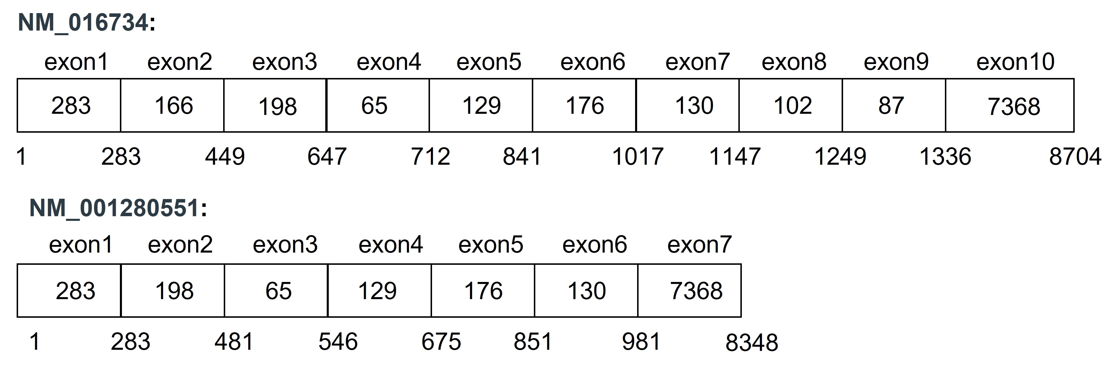
We want to study expression levels of Pax5 transcript variant 1 (NM_016734). The first step is to design specific primers for this transcript. To increase specificity the forward and the reverse primers are located on two adjacent exons of the transcript (Figure 63, green arrows). This increases the chance of a single specific product:

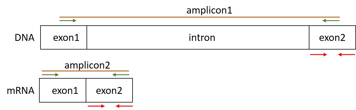
Figure 63: Primer design for gene expression analysis

If there was contamination of DNA in your original RNA sample the PCR product based on the DNA sequence becomes too long to amplify (amplicon1). In the case of mRNA, a short amplicon (amplicon2) is created because the intron is no longer present in the mRNA and thus the final cDNA). The optimal length for an amplicon in a qPCR reaction is between 80-125 bp. Thus, in case you design primers within a single exon you don’t know whether the signal comes from DNA or mRNA (Figure 63, red arrows).

lesson_06_assignment

Obtain the coordinates of exon1 en exon2 of the Pax5 NM_016734 transcript.
(This is needed for the next assignment to design primers)

HINT: use NCBI nucleotide database

NCBI primer blast

There are several online resources to design primers. Here we will use the NCBI primer blast tool. To design primers we have to provide a nucleotide sequence, in this case the NM_016734 transcript of Pax5 (Figure 64).

To design the forward primer in exon1 and the reverse primer in exon2:

provide the coordinates of exon1 in the range field (begin, end) (see assignment_2)
provide the coordinates of exon2 in the range field (begin, end) (see assignment_2)

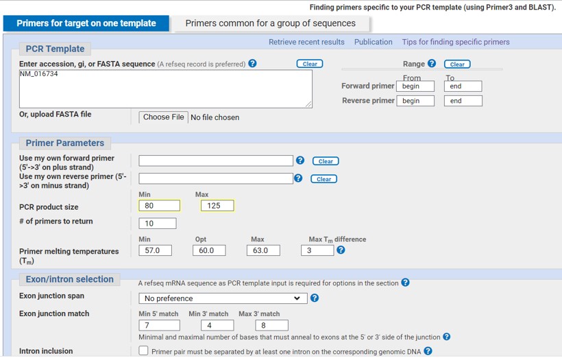
Figure 64: NCBI primer blast

Fill out the PCR product size as shown in Figure 64 (80-125)
Use the standard default for the other parameters
Click on “Get Primers” (can take up to minute)

The program will first show other Pax5 transcripts that are highly similar to the NM_016734 transcript. Exclude those transcripts (default) and continue

After the program is done you will find a list of primer pairs that can be used for qRT-PCR (Figure 65)

The output provide the following information:
- The length of the primers
- Start and stop position within the sequence
- Melt temperature (Tm) which should be quit similar
- Percentage GC (how many C and G are present in the primer sequence)
- Self complementary: the lower the number the better
- Self 3’ complementary: the lower the number the better

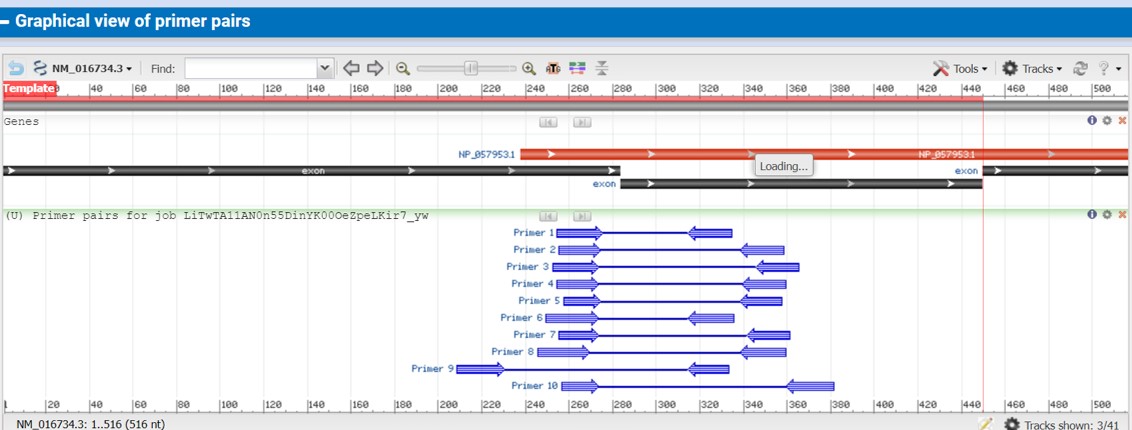
Figure 65: NCBI primer blast output

We can select set of primers and send those sequences to a company that will synthesise the primers. It is important to note that on forehand you don’t know whether your primers will produce a specific result. You can only find out when doing the qRT-PCR experiment and analyze the results!!

lesson_06_assignment

The Pax5 gene produces different transcripts. You have already designed primers for Pax5 transcript NM_016734 (isoform 1). After reading the literature you decided to measure expression levels of Pax5 transcript NM_016734 (isoform6). Transcript isoform6 lacks three exons compared to isoform1

Design specific primers for Pax5 transcript1 and transcript6 meaning that primers for transcript1 should only amplify transcript1 (and not transcript6) and primers for transcript6 should only amplify transcript6 (and not transcript1)

HINT: Carefully think which exons you want to include for primer design for each transcript

Design primers for a house keeping gene for data normalization. Choose your own gene. Search on the internet for a list of house keeping genes (in combination with qRT-PCR) and use the NCBI gene and nucleotide databases to obtain exon sequence information. Use NCBI primer blast to design the primers.

qRT-PCR data analysis

After designing the primers, mRNA isolation, conversion of mRNA to cDNA and the qPCR reaction you obtained a set of Ct values. The results are in file lesson_06_opdracht4_student.csv. The file is located in the data folder on the server

lesson_06_assignment

Data inspection

How many biological replicates are measured in each group?
How many technical replicates are measured for each person?

Open the file in JASP

lesson_06_assignment

Descriptive statistics in JASP

Calculate the average and standard deviation of the technical replicates for each transcript per person
What is your conclusion. Is there a lot of noise in the data due to the protocol and equipment?
Calculate the average and standard deviation of the two groups for each transcript
Include a boxplot in the descriptive analysis (Plots -> Boxplots)
What is your conclusion?

After the data inspection in JASP we perform the \(\Delta\Delta\)Ct method in Excel

lesson_06_assignment

Data transformation, organisation and analysis

Import the file lesson_06_opdracht4_student.csv in Excel
Analyse the data using the \(\Delta\Delta\)Ct method
Create a complete graph to visualize your data
Statistically test for each transcript whether there is a difference in normalized average Ct values between the Control and the ALL group

RNA-seq

With the recent advances of high-throughput DNA sequencing techniques it is possible to simultaneously measure the transcripts levels of all genes in cells in stead of a limited set of genes using a qRT-PCR reaction. Because you don’t have to make a prior selection of genes that you want to test, the RNA-seq approach is unbiased. Similar to the qRT-PCR protocol, mRNA is isolated from selected cells and converted to cDNA. An important step is to make smaller fragments of the cDNA. The cDNA is subsequenctly prepared in such a way that millions of cDNA fragments can be sequenced in parallel in one experiment. The output of an RNA-seq experiment consists of millions of sequenced cDNA reads stored in a gigantic FASTA-like file called a FASTQ file. To identify the transcripts (from which gene they were transcribed) the sequences are aligned ( = compared to the genome of the cells from where the mRNA was isolated) using special bioinformatics tools.

Read the first section 0 of this RNA-seq information page

The next step is to count how many sequence reads were aligned to a certain gene. This could be expressed as RPMK (read per million per kilobase). This procedures involves several normalization steps:

Imagine we have two sample:

Sample A: 10,8 million sequenced reads Sample B: 17,3 million sequenced reads

The total number of reads for each experiment is called the sequencing depth. The sequencing depth depends on how good the experiment was performed and this is a technical differences. Thus the first step is to normalize the number of reads associated with a gene for the differences in sequencing depth:

Calculate the sequencing depth scaling factor = total number of reads divided by a million
- sample A: 10,8
- sample B: 17,3
Divide the number of reads associated with a gene by the scaling factor -> Reads per million (RPM)

Each gene produces an mRNA transcript of a certain length. Longer mRNA molecules generate more reads to start with. Thus, we also normalize for the gene length

Divide the RPM by the gene length in kilobase (kbp = 1000 bp) -> Read per million per kilobase (RPMK)

(To make it even more complicated another unit of RNA-seq gene expression is TPM. Here, the number of reads per gene is first divided by the length of the gene and secondly by the scaling factor. This unit is called TPM (Transcripts Per Kilobase Million) and has different properties compared to RPMK

NOTE: If you are interested in the complete RNA-seq data analysis pipeline you can enter the Data Science specialization courses in VL5/6

After processing the raw sequencing data you end up with a list of about 20.000 protein coding genes with their normalized transcript count.

A researcher is studying the gene expression profiles in mouse B cells and macrophages. The data is in file lesson6_opdracht7.txt. The file consist of three columns:

transcript identifier
Normalized reads B cells
Normalized reads macrophages

Genes that are expressed at low levels (values of < 10 in both B cells and macrophages) are removed. The dataset only contains genes which show a difference in gene expression between B cells and macrophages of more then two-fold.

lesson_06_assignment

Data inspection transformation and descriptive statistics

Import the file lesson_06_opdracht7_student.txt in JASP
Name the Descriptive tab in JASP “lesson6_opdracht7”

How many genes are present in the data file?
What are the mean, median and standard deviation?
Why is there such a big difference between the mean and the median?

To reduce the range of gene expression values, these values are often logarithmic transformed.

Create two extra columns in JASP with the log10 transformed values of column Reads_Bcells and Reads_Mac

lesson_06_assignment

Open a new Descriptive tab in JASP and name the tab “lesson6_opdracht8”

What are the mean, median and standard deviation of the log10 transformed gene expression values in B cells and macrophages?
Are the log10 transformed expression values in B cells and macrophages normally distributed?

Create a Scatter plot -> Interpret the scatter plot

The genes below the diagonal are higher / lower expressed in B cells compared to macrophages?
The genes above the diagonal are higher / lower expressed in B cells compared to macrophages?

To identify genes that show a difference in gene expression between B cells and macrophages we calculate the difference between the log10 values. This means that a difference of 1 between the log10 expression values of B cells and macrophages translate to 10¹ = 10 fold difference.

Create an extra column in JASP and calculate the difference between log10 transformed values of Bcells and macrophages (Bcells - macrophages)

lesson_06_assignment

Open a new Descriptive tab in JASP and name the tab “lesson6_opdracht9”

Calculate the quartiles of the difference in gene expression on the log transformed values (= last column)
Create a Distribution plot of the values of the last column

To count how many genes are upregulated and downregulated in Bcells compared to macrophages we have to count the number of genes that have a difference in log10 expression value bigger or smaller then 0.
Filter genes with values > 0 and count the number of genes
Filter genes with values < 0 and count the number of genes

How many genes show higher expression values in B cells compared to macrophages?
How many genes show lower expression values in B cells compared to macrophages?

Inspect the last column and note that the list of expression values was already sorted:

What is the gene name of the gene that shows highest expression in macrophages compared to B cells?